Pytorch:Convolutional Neural Network-LeNet
Copyright: Jingmin Wei, Pattern Recognition and Intelligent System, School of Artificial and Intelligence, Huazhong University of Science and Technology
This tutorial is not commercial and is only for learning and reference exchange. If you need to reproduce it, please contact me.
In Multilayer Perceptors, we construct a Multilayer Perceptors model with a single hidden layer to perform classification and regression tasks. However, this classification method has some limitations.
Pixels adjacent to the image in the same column may be far apart in this vector. The patterns they form may be difficult to identify by the model.
For large-sized input images, the use of full-connection layers can easily cause the model to be too large. Assume that both the height and width of the input are 1000 1000 1000 pixel color photograph (including 3 3 3 channels). Even though the number of full connection layer outputs is still 256 256 256, the shape of the layer weight parameter is 3000000 × 2563000000 × 256 3000000\times2563000000\times256 3000000 × 2563000000 × 256: It takes up about 3 3 3 GB of memory or video memory. This results in complex models and high storage overhead.
The convolution layer tries to solve both problems. On the one hand, the convolution layer retains the input shape so that the correlation between the pixels of the image in both the width and height directions may be effectively identified. On the other hand, the convolution layer recalculates the same convolution kernel with inputs from different locations through a sliding window, thus avoiding the parameter size being too large.
A convolution network is a network with convolution layers. In this section, we will introduce a convolution neural network, LeNet, that was used earlier to recognize handwritten digital images. The name comes from Yann LeCun, the first author of LeNet's paper. LeNet shows that training a convolution neural network with gradient descent is the most advanced way to recognize handwritten numbers at that time. For the first time, this groundbreaking work has brought convolution neural networks to the stage.
Lenet Model
LeNet is divided into convolution layer blocks and fully connected layer blocks. Below we will describe the two modules separately.
The basic unit in a convolution layer block is the maximum pooled layer after the convolution layer: the convolution layer is used to identify spatial patterns in the image, such as lines and object localities, and the maximum pooled layer after the convolution layer is used to reduce the location sensitivity of the convolution layer. Convolutional layer blocks consist of two such basic units stacked repeatedly. In convolution layer blocks, each convolution layer is used 5 × 55 × 5 5×55×5 5 × 55 × 5 window, and use sigmoid activation function on the output. The number of output channels for the first convolution layer is 6 6 6, the number of output channels for the second convolution layer increases to 16 16 16. This is because the input height and width of the second convolution layer are smaller than the input of the first convolution layer, so increasing the output channel makes the parameter sizes of the two convolution layers similar. The window shapes of the two largest pooled layers of a convolution block are both 2 × 22 × 2 2×22×2 2 × 22 × 2 with steps of 2 2 2. Since the pooled window has the same shape as the step, the areas covered by each slide of the pooled window on the input do not overlap.
The output shape of the convolution layer block is (batch size, channel, height, width). When the output of a convolution layer block is passed into a fully connected layer block, the fully connected layer block flattens each sample in a small batch. That is, the input shape of the fully connected layer becomes two-dimensional, where the first dimension is the sample in a small batch and the second dimension is the vector representation of each sample flattened, and the vector length is the product of the channel, height and width. Fully connected layer block contains 3 3 Three fully connected layers. Their output numbers are 120 120 120 , 84 84 84 and 10 10 10, where 10 10 10 is the number of categories output.
import numpy as np
import pandas as pd
from sklearn.metrics import accuracy_score, confusion_matrix
import matplotlib.pyplot as plt
import seaborn as sns
import copy
import time
import torch
import torch.nn as nn
from torch.optim import Adam
import torch.utils.data as Data
from torchvision import transforms
from torchvision.datasets import FashionMNIST
# Model Load Selection GPU
device = torch.device("cuda" if torch.cuda.is_available() else "cpu")
print(device)
print(torch.cuda.device_count())
print(torch.cuda.get_device_name(0))
cuda
1
GeForce MX250
Image data preparation
API function read that calls FashionMNIST of sklearn s datasets module.
# Prepare training datasets using FashionMNIST data
train_data = FashionMNIST(
    root = './data/FashionMNIST',
    train = True,
    transform = transforms.ToTensor(),
    download = False
)

# Define a data loader
train_loader = Data.DataLoader(
    dataset = train_data,   # data set
    batch_size = 64,    # Size of batch processing
    shuffle = False,   # Do not clutter data
    num_workers = 2,    # Two processes
)

# Calculate batch number
print(len(train_loader))
938
The above block defines a data loader with 64 data blocks in batch.
Next, we do data visualization analysis, convert tensor data to numpy format, and visualize it using imshow.
# Get batch data

for step, (b_x, b_y) in enumerate(train_loader):
    if step > 0:
        break
# Visualize an image of a batch
batch_x = b_x.squeeze().numpy()
batch_y = b_y.numpy()
label = train_data.classes
label[0] = 'T-shirt'

plt.figure(figsize = (12, 5))
for i in np.arange(len(batch_y)):
    plt.subplot(4, 16, i + 1)
    plt.imshow(batch_x[i, :, :], cmap = plt.cm.gray)
    plt.title(label[batch_y[i]], size = 9)
    plt.axis('off')
    plt.subplots_adjust(wspace = 0.05)
# Processing Test Sets
test_data = FashionMNIST(
    root = './data/FashionMNIST',
    train = False, # Do not use training datasets
    download = False
)

# Add a channel dimension to the data and normalize the range of values
test_data_x = test_data.data.type(torch.FloatTensor) / 255.0
test_data_x = torch.unsqueeze(test_data_x, dim = 1)
test_data_y = test_data.targets # Test Set Label

print(test_data_x.shape)
print(test_data_y.shape)
torch.Size([10000, 1, 28, 28])
torch.Size([10000])
Building LeNet Convolution Neural Network
class LeNet(nn.Module):
    def __init__(self):
        super(LeNet, self).__init__()
        self.conv = nn.Sequential(
            nn.Conv2d(1, 6, 5), # in_channels, out_channels, kernel_size
            nn.Sigmoid(),
            nn.MaxPool2d(2, 2), # kernel_size, stride
            nn.Conv2d(6, 16, 5),
            nn.Sigmoid(),
            nn.MaxPool2d(2, 2)
        )
        self.fc = nn.Sequential(
            nn.Linear(16*4*4, 120),
            nn.Sigmoid(),
            nn.Linear(120, 84),
            nn.Sigmoid(),
            nn.Linear(84, 10)
        )

    def forward(self, img):
        feature = self.conv(img)
        output = self.fc(feature.view(img.shape[0], -1))
        return output
# Define convolution network objects
mylenet = LeNet().to(device)
from torchsummary import summary
summary(mylenet, input_size=(1, 28, 28))
----------------------------------------------------------------
        Layer (type)               Output Shape         Param #
================================================================
            Conv2d-1            [-1, 6, 24, 24]             156
           Sigmoid-2            [-1, 6, 24, 24]               0
         MaxPool2d-3            [-1, 6, 12, 12]               0
            Conv2d-4             [-1, 16, 8, 8]           2,416
           Sigmoid-5             [-1, 16, 8, 8]               0
         MaxPool2d-6             [-1, 16, 4, 4]               0
            Linear-7                  [-1, 120]          30,840
           Sigmoid-8                  [-1, 120]               0
            Linear-9                   [-1, 84]          10,164
          Sigmoid-10                   [-1, 84]               0
           Linear-11                   [-1, 10]             850
================================================================
Total params: 44,426
Trainable params: 44,426
Non-trainable params: 0
----------------------------------------------------------------
Input size (MB): 0.00
Forward/backward pass size (MB): 0.08
Params size (MB): 0.17
Estimated Total Size (MB): 0.25
----------------------------------------------------------------
# Output Network Structure
from torchviz import make_dot

x = torch.randn(1, 1, 28, 28).requires_grad_(True)
y = mylenet(x.to(device))
myCNN_vis = make_dot(y, params=dict(list(mylenet.named_parameters()) + [('x', x)]))
myCNN_vis
LeNet Network Training and Prediction
The training set as a whole has 60000 60000 60,000 images, 938 938 938 batch es, using 80 % 80\% 80% of batch es are used for model training. 20 % 20\% 20% for model validation
# Define network training process functions
def train_model(model, traindataloader, train_rate, criterion, optimizer, num_epochs = 25):
    '''
    Model, training dataset(To be sliced),Percentage of training set, loss function, optimizer, number of training rounds
    '''
    # Calculate the number of batch es used for training
    batch_num = len(traindataloader)
    train_batch_num = round(batch_num * train_rate)
    # Copy model parameters
    best_model_wts = copy.deepcopy(model.state_dict())
    best_acc = 0.0
    train_loss_all = []
    val_loss_all =[]
    train_acc_all = []
    val_acc_all = []
    since = time.time()
    # Training Framework
    for epoch in range(num_epochs):
        print('Epoch {}/{}'.format(epoch, num_epochs - 1))
        print('-' * 10)
        train_loss = 0.0
        train_corrects = 0
        train_num = 0
        val_loss = 0.0
        val_corrects = 0
        val_num = 0
        for step, (b_x, b_y) in enumerate(traindataloader):
            b_x, b_y = b_x.to(device), b_y.to(device)
            if step < train_batch_num:
                model.train()   # Set as training mode
                output = model(b_x)
                pre_lab = torch.argmax(output, 1)
                loss = criterion(output, b_y)   # Calculating Error Loss
                optimizer.zero_grad()   # Empty Past Gradient
                loss.backward() # Error Back Propagation
                optimizer.step()    # Update parameters based on errors
                train_loss += loss.item() * b_x.size(0)
                train_corrects += torch.sum(pre_lab == b_y.data)
                train_num += b_x.size(0)
            else:
                model.eval()    # Set to Verification Mode
                output = model(b_x)
                pre_lab = torch.argmax(output, 1)
                loss = criterion(output, b_y)
                val_loss += loss.cpu().item() * b_x.size(0)
                val_corrects += torch.sum(pre_lab == b_y.data)
                val_num += b_x.size(0)
        # ==========================End of small loop=======================End of small loop==========

        # Calculate loss and accuracy of an epoch on training and validation sets
        train_loss_all.append(train_loss / train_num)
        train_acc_all.append(train_corrects.double().item() / train_num)
        val_loss_all.append(val_loss / val_num)
        val_acc_all.append(val_corrects.double().item() / val_num)
        print('{} Train Loss: {:.4f} Train Acc: {:.4f}'.format(epoch, train_loss_all[-1], train_acc_all[-1]))
        print('{} Val Loss: {:.4f} Val Acc: {:.4f}'.format(epoch, val_loss_all[-1], val_acc_all[-1]))

        # Parameters with the highest precision of the copy model
        if val_acc_all[-1] > best_acc:
            best_acc = val_acc_all[-1]
            best_model_wts = copy.deepcopy(model.state_dict())
        time_use = time.time() - since
        print('Train and Val complete in {:.0f}m {:.0f}s'.format(time_use // 60, time_use % 60))
    # ===============================End of Big Loop==========================


    # Parameters using the best model
    model.load_state_dict(best_model_wts)
    train_process = pd.DataFrame(
        data = {'epoch': range(num_epochs),
                'train_loss_all': train_loss_all,
                'val_loss_all': val_loss_all,
                'train_acc_all': train_acc_all,
                'val_acc_all': val_acc_all})
    return model, train_process
Loss of model and recognition accuracy make up data table train_process output, using copy.deepcopy() saves the optimal parameters of the model in best_ Model_ In the wts, all the final training results pass the model.load_state_dict(best_model_wts) assigns the optimal parameters to the final model
The following are training models and optimizers:
# model training
optimizer = Adam(mylenet.parameters(), lr = 0.001)   # Adam Optimizer
criterion = nn.CrossEntropyLoss()   # loss function
myconvnet, train_process = train_model(mylenet, train_loader, 0.8, criterion, optimizer, num_epochs = 25)
Epoch 0/24
----------
0 Train Loss: 1.3207 Train Acc: 0.5002
0 Val Loss: 0.8333 Val Acc: 0.6904
Train and Val complete in 0m 16s
Epoch 1/24
----------
1 Train Loss: 0.7443 Train Acc: 0.7220
1 Val Loss: 0.6562 Val Acc: 0.7502
Train and Val complete in 0m 29s
Epoch 2/24
----------
2 Train Loss: 0.6337 Train Acc: 0.7557
2 Val Loss: 0.5853 Val Acc: 0.7726
Train and Val complete in 0m 43s
Epoch 3/24
----------
3 Train Loss: 0.5743 Train Acc: 0.7765
3 Val Loss: 0.5447 Val Acc: 0.7833
Train and Val complete in 0m 55s
Epoch 4/24
----------
4 Train Loss: 0.5339 Train Acc: 0.7921
4 Val Loss: 0.5160 Val Acc: 0.7925
Train and Val complete in 1m 7s
Epoch 5/24
----------
5 Train Loss: 0.5021 Train Acc: 0.8060
5 Val Loss: 0.4914 Val Acc: 0.8082
Train and Val complete in 1m 19s
Epoch 6/24
----------
6 Train Loss: 0.4777 Train Acc: 0.8157
6 Val Loss: 0.4719 Val Acc: 0.8207
Train and Val complete in 1m 32s
Epoch 7/24
----------
7 Train Loss: 0.4583 Train Acc: 0.8266
7 Val Loss: 0.4565 Val Acc: 0.8271
Train and Val complete in 1m 45s
Epoch 8/24
----------
8 Train Loss: 0.4416 Train Acc: 0.8341
8 Val Loss: 0.4432 Val Acc: 0.8324
Train and Val complete in 1m 56s
Epoch 9/24
----------
9 Train Loss: 0.4264 Train Acc: 0.8410
9 Val Loss: 0.4308 Val Acc: 0.8387
Train and Val complete in 2m 7s
Epoch 10/24
----------
10 Train Loss: 0.4128 Train Acc: 0.8455
10 Val Loss: 0.4191 Val Acc: 0.8434
Train and Val complete in 2m 18s
Epoch 11/24
----------
11 Train Loss: 0.4006 Train Acc: 0.8498
11 Val Loss: 0.4083 Val Acc: 0.8475
Train and Val complete in 2m 30s
Epoch 12/24
----------
12 Train Loss: 0.3896 Train Acc: 0.8540
12 Val Loss: 0.3983 Val Acc: 0.8503
Train and Val complete in 2m 43s
Epoch 13/24
----------
13 Train Loss: 0.3795 Train Acc: 0.8580
13 Val Loss: 0.3894 Val Acc: 0.8531
Train and Val complete in 2m 53s
Epoch 14/24
----------
14 Train Loss: 0.3704 Train Acc: 0.8614
14 Val Loss: 0.3812 Val Acc: 0.8552
Train and Val complete in 3m 3s
Epoch 15/24
----------
15 Train Loss: 0.3621 Train Acc: 0.8641
15 Val Loss: 0.3739 Val Acc: 0.8582
Train and Val complete in 3m 14s
Epoch 16/24
----------
16 Train Loss: 0.3545 Train Acc: 0.8669
16 Val Loss: 0.3674 Val Acc: 0.8613
Train and Val complete in 3m 25s
Epoch 17/24
----------
17 Train Loss: 0.3474 Train Acc: 0.8696
17 Val Loss: 0.3615 Val Acc: 0.8628
Train and Val complete in 3m 36s
Epoch 18/24
----------
18 Train Loss: 0.3409 Train Acc: 0.8720
18 Val Loss: 0.3563 Val Acc: 0.8652
Train and Val complete in 3m 47s
Epoch 19/24
----------
19 Train Loss: 0.3347 Train Acc: 0.8742
19 Val Loss: 0.3516 Val Acc: 0.8678
Train and Val complete in 3m 58s
Epoch 20/24
----------
20 Train Loss: 0.3289 Train Acc: 0.8761
20 Val Loss: 0.3473 Val Acc: 0.8699
Train and Val complete in 4m 10s
Epoch 21/24
----------
21 Train Loss: 0.3234 Train Acc: 0.8783
21 Val Loss: 0.3434 Val Acc: 0.8718
Train and Val complete in 4m 22s
Epoch 22/24
----------
22 Train Loss: 0.3182 Train Acc: 0.8803
22 Val Loss: 0.3397 Val Acc: 0.8742
Train and Val complete in 4m 36s
Epoch 23/24
----------
23 Train Loss: 0.3132 Train Acc: 0.8821
23 Val Loss: 0.3362 Val Acc: 0.8761
Train and Val complete in 4m 47s
Epoch 24/24
----------
24 Train Loss: 0.3085 Train Acc: 0.8838
24 Val Loss: 0.3331 Val Acc: 0.8771
Train and Val complete in 4m 58s
# Visual training process
plt.figure(figsize = (12, 4))
plt.subplot(1, 2, 1)
plt.plot(train_process.epoch, train_process.train_loss_all, 'ro-', label = 'Train loss')
plt.plot(train_process.epoch, train_process.val_loss_all, 'bs-', label = 'Val loss')
plt.legend()
plt.xlabel('epoch')
plt.ylabel('Loss')

plt.subplot(1, 2, 2)
plt.plot(train_process.epoch, train_process.train_acc_all, 'ro-', label = 'Train acc')
plt.plot(train_process.epoch, train_process.val_acc_all, 'bs-', label = 'Val acc')
plt.legend()
plt.xlabel('epoch')
plt.ylabel('Acc')

plt.show()
At the same time, we calculate the generalization ability of the model and use the output model to make predictions on the test set:
# Test Set Prediction and Visualize Prediction Effect
mylenet.eval()
output = mylenet(test_data_x.to(device))
pre_lab = torch.argmax(output, 1)
acc = accuracy_score(test_data_y, pre_lab.cpu())
print(test_data_y)
print(pre_lab)
print('The prediction accuracy on the test set is', acc)
tensor([9, 2, 1,  ..., 8, 1, 5])
tensor([9, 2, 1,  ..., 8, 1, 5], device='cuda:0')
Prediction accuracy on test set is 0.8677
# Compute and visualize confusion matrices on test sets
conf_mat = confusion_matrix(test_data_y, pre_lab.cpu())
df_cm = pd.DataFrame(conf_mat, index = label, columns = label)
heatmap = sns.heatmap(df_cm, annot = True, fmt = 'd', cmap = 'YlGnBu')
heatmap.yaxis.set_ticklabels(heatmap.yaxis.get_ticklabels(), rotation = 0, ha = 'right')
heatmap.xaxis.set_ticklabels(heatmap.xaxis.get_ticklabels(), rotation = 45, ha = 'right')
plt.ylabel('True label')
plt.xlabel('Predicted label')
plt.show()
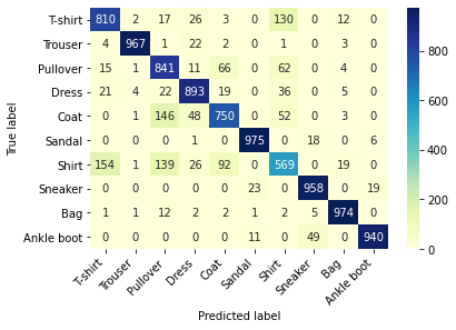
We find that T-shirt and Shirt are the easiest predictors of errors, and the sample size of each prediction error is 154 154 154.