Pytoch: image style migration
Copyright: Jingmin Wei, Pattern Recognition and Intelligent System, School of Artificial and Intelligence, Huazhong University of Science and Technology
Reference
Image Style Transfer Using Convolutional Neural Networks
A Neural Algorithm of Artistic Style
Perceptual Losses for Real-Time Style Transfer and Super-Resolution
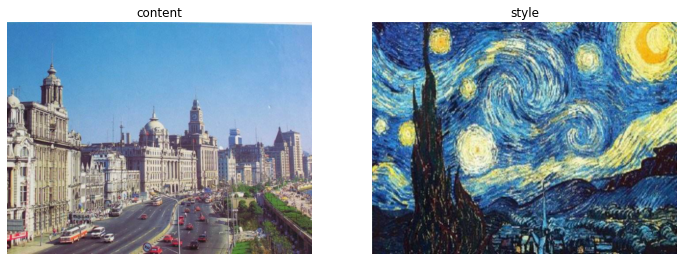
The main task of image style migration is to migrate the image style to the content image, so that the content image also has a certain style.
Style images can be some works of artists, including the style of artists, or classic photos with distinctive colors. Content images usually come from the real world.
Using style migration, the content image can be processed into the desired style.
Common image style migration methods
Common style migration of fixed content
Reference article:
Image Style Transfer Using Convolutional Neural Networks
A Neural Algorithm of Artistic Style
The idea is to take the picture as a variable that can be trained. By continuously optimizing the pixel value of the picture, reduce the content difference between the picture and the content picture, and reduce the style difference between the picture and the style picture. Through multiple iterative training of the convolution network, an image with a specific style can be generated. The style of the generated content is consistent with that of the picture.
The image style migration based on the convolution layer in VGG16 network is as follows: a ⃗ \vec{a} a For the input style image, p ⃗ \vec{p} p Image for the input content, x ⃗ \vec{x} x It is the image after the image style migration generated by random noise. L c o n t e n t \mathcal{L}_{content} Lcontent indicates the loss of image content, L s t y l e \mathcal{L}_{style} Lstyle indicates the style loss of the image, α \alpha α and β \beta β Represent content loss weight and style loss weight respectively.
The feature map calculated by deeper convolution can better represent the image content, while the feature map calculated by shallow convolution can better represent the image style. Based on this, we can measure the style, content and style of the target image through the feature map of different convolution layers.
The content similarity measurement of the two images is mainly through in conv4_ The similarity of feature mapping on layer 2 is regarded as content loss
L c o n t e n t = 1 2 ∑ i , j ( F i j l − P i j l ) 2 \mathcal{L}_{content} = \frac{1}{2}\sum_{i,j}(F_{ij}^l-P_{ij}^l)^2 Lcontent=21i,j∑(Fijl−Pijl)2
l l l represents the number of layers of feature mapping, F F F and P P P is the feature mapping of the target image and eirong image output in the pronunciation volume layer respectively.
The style loss of two images is not directly compared through feature mapping, but the style of the image is calculated by calculating the Gram matrix and compared. The Gram matrix for calculating the feature mapping is to transform its feature mapping into a column vector, and the Gram matrix is obtained by multiplying the column vector by its transpose, which can better represent the style of the image. So input style image a ⃗ \vec{a} a And target image x ⃗ \vec{x} x use A l A^l Al and G l G^l Gl indicates that they are in l l For the style representation of l-layer feature mapping (the calculated Gram matrix), the style loss of the image can be calculated in the following way:
E l = 1 4 N l 2 M l 2 ∑ i , j ( G i j l − A i j l ) 2 L s t y l e = ∑ l = 0 L w l E l E_l = \frac{1}{4N_l^2M_l^2}\sum_{i,j}(G_{ij}^l-A_{ij}^l)^2\\ \mathcal{L}_{style} = \sum_{l=0}^Lw_lE_l El=4Nl2Ml21i,j∑(Gijl−Aijl)2Lstyle=l=0∑LwlEl
w l w_l wl is the weight of the style loss of each layer, N l N_l Nl # and M l M_l Ml ^ corresponds to the height and width of the feature map.
Fast style migration of fixed style and arbitrary content
Reference article:
Perceptual Losses for Real-Time Style Transfer and Super-Resolution
That is to add an image conversion network for training on the basis of ordinary image style migration. After training for a style image, any input image can be transferred and learned very quickly, so that the image has a good learning image style.
The network can be seen as two parts. One part is through the input image x x x through image conversion network f w fw fw, get the output of the network y ^ \hat{y} y ^, this part is not in the framework of ordinary style migration image. The input image of ordinary apology is random noise, while the input image of fast style migration is an image through the conversion network f w fw fw output. Another part of the network uses the correlation convolution layer in VGG16 network to measure the content loss and style loss of an image.
In the image conversion network part, it can be divided into 3 3 There are three stages: image dimensionality reduction, residual connection and image dimensionality upgrading.
Image dimensionality reduction: 3 3 3 convolution layers, 256 × 256 → 64 × 64 256\times256\rightarrow 64\times64 two hundred and fifty-six × 256→64 × 64, number of channels 3 → 128 3\rightarrow128 3→128 .
Residual connection: 5 5 5 residual blocks to learn the image, learn how to add a small amount of content to the original image and change the style of the original image.
The main idea is to assume that there is a network M M M. Output as X X 10. If to the network M M M adds a layer of network called sex M n e w M_{new} Mnew, whose output is H ( X ) H(X) H(X) . The design idea of residual connection is to ensure the network M n e w M_{new} Mnew's performance ratio network M M M strong, make the network M n e w M_{new} The output of Mnew is H ( X ) = F ( X ) + X H(X)=F(X)+X H(X)=F(X)+X , M n e w M_{new} Mnew is guaranteeing M M Output of M X X At the same time of X, a residual output is added F ( X ) F(X) F(X), so as long as the residual learning is more than "identical to" 0 0 0 "if the function is better, the network can be guaranteed M n e w M_{new} Mnew's effect must be better than the network M M M OK.
Image dimension upgrading: output 5 5 Unit, 5 residuals 3 3 The operation of three convolution layers gradually reduces the number of channels from 128 128 128 shrink to 3 3 3. The mapping size of each feature is from 64 × 64 64\times64 sixty-four × 64 zoom in to 256 × 256 256\times256 two hundred and fifty-six × 256, transpose convolution can also be used to complete the dimension upgrading part.
For fast style migration, in addition to content loss and style loss, total variational loss can also be used to smooth the image.
Common style migration of fixed content
from PIL import Image
import matplotlib.pyplot as plt
import numpy as np
import requests
import time
import hiddenlayer as hl
from skimage.io import imread

import torch
from torchvision import transforms
import torch.optim as optim
from torchvision import models
# Select GPU for model loading
# device = torch.device("cuda" if torch.cuda.is_available() else "cpu")
device = torch.device('cpu')
print(device)
print(torch.cuda.device_count())
print(torch.cuda.get_device_name(0))
cpu
1
GeForce MX250
Prepare VGG19 network
In order to speed up the network training process, it is not necessary to update the parameter weight of VGG19, and freeze its weight after import.
vgg19 = models.vgg19(pretrained = True).to(device)
# There is no need for network classifier, only convolution and pooling layer
vgg = vgg19.features
# Freeze the network weight and do not update it during training
for param in vgg.parameters():
    param.requires_grad_(False)
Image data preparation
Control the size of the image in advance in order to speed up the style migration.
The first parameter is the read path, and the second and third parameters control the image size.
If Max is specified_ Size, read the image. If the image size is too large, the image will be reduced accordingly. If shape is specified, the image is converted to shape size.
def load_image(img_path, max_size = 400, shape = None):
    '''
    Read the image and ensure that the height and width of the image are less than 400 by default
    '''
    image = Image.open(img_path)
    # If the image size is too large, size conversion is performed
    if max(image.size) > max_size:
        size = max_size
    else:
        size = max(image.size)
    # If an image size is specified, the image is converted to the size specified by shape
    if shape is not None:
        size = shape
    # Use transforms to convert the image into tensor and standardize it
    in_transform = transforms.Compose(
        [transforms.Resize(size), # Image size transformation, short edge matching
         transforms.ToTensor(), # Turn into tensor
         # Image standardization
         transforms.Normalize((0.485, 0.456, 0.406),
                              (0.229, 0.224, 0.225))])
    # Use the RGB channel of the image and add the batch dimension
    image = in_transform(image)[:3, :, :].unsqueeze(dim = 0)
    return image
Define an im_ The covert function converts the four-dimensional tensor of an image into a three-dimensional array that can be visualized using the matplotlib library.
def im_convert(tensor):
    '''
    take[1, c, h, w]The tensor of dimension is transformed into[h, w, c]Array of
    Because the tensor is standardized, the standardized inverse transformation is required
    '''
    image = tensor.data.numpy().squeeze() # Remove batch dimension data
    image = image.transpose(1, 2, 0) # Permutation array dimension [C, h, w] - [h, W, C]
    # Conduct standardized reverse operation
    image = image * np.array((0.229, 0.224, 0.225)) + np.array((0.485, 0.456, 0.406))
    image = image.clip(0, 1) # Cut the value of the image to 0-1
    return image
# Read content and style images
content = load_image('./data/styletransfer/buildings1.png', max_size = 400)
print('content shape:', content.shape)
# Set the width and height of the style image according to the width and height of the content image
style = load_image('./data/styletransfer/starry-sky1.png', shape = content.shape[-2: ])
print('style shape:', style.shape)
# Visual content image and style image
fig, (ax1, ax2) = plt.subplots(1, 2, figsize = (12, 5))
ax1.imshow(im_convert(content))
ax1.set_title('content')
ax2.imshow(im_convert(style))
ax2.set_title('style')
ax1.axis('off')
ax2.axis('off')
plt.show()
content shape: torch.Size([1, 3, 400, 526])
style shape: torch.Size([1, 3, 400, 526])
Output characteristics of image and calculation of Gram matrix
The feature mapping of the output image on the specified network layer, and the output results are saved in a dictionary.
# Used to obtain the output of the specified layer of the image on the network
def get_features(image, model, layers = None):
    '''
    The image propagates forward and obtains the feature mapping to the top layer
    '''
    # The full mapping layer name of VGGnet of torch corresponds to the name in the paper
    # The layers parameter specifies the layer that needs to be used for the content and style representation of the image
    # If layers is not specified, the default layer is used
    if layers is None:
        layers = {'0': 'conv1_1',
                  '5': 'conv2_1',
                  '10': 'conv3_1',
                  '19': 'conv4_1',
                  '21': 'conv4_2', # Representation of content layers
                  '28': 'conv5_1'}
    features = {} # The acquired features of each layer are saved in the dictionary
    x = image.to(device) # The image of the feature needs to be acquired
    # model._modules is a dictionary that holds the information of each layer of the network model
    for name, layer in model._modules.items():
        # Acquire image features from the first layer
        x = layer(x)
        # If it is the feature specified by the layers parameter, it is saved to features
        if name in layers:
            features[layers[name]] = x
    return features
When comparing whether two images have the same style, you can use Gram matrix to evaluate:
For the input four-dimensional feature map, set each feature map as a vector to obtain a matrix with behavior D (number of feature maps) listed as h * w (number of pixels per feature map), which is multiplied by its transpose to obtain the required Gram matrix.
def gram_matrix(tensor):
    '''
    Calculates the of the specified vector Gram Matrix, The matrix represents the style features of the image
    Gram matrix can finally transmit the style under the condition of ensuring the content
    tensor: It is a layer of feature mapping after forward calculation of an image
    '''
    # Obtain the batch of tensor_ size, depth, height, width
    _, d, h, w = tensor.size()
    # Change the dimension of the matrix
    tensor = tensor.view(d, h * w)
    # Calculate gram matrix
    gram = torch.mm(tensor, tensor.t())
    return gram
Calculate the feature output for the content image and style image, and calculate the Gram matrix of the style image on each feature output.
At the same time, create a target image, which finally needs to generate a content image with style, that is, the final output.
# Calculate the style representation of content image
content_features = get_features(content, vgg)
# Style representation of computational style image
style_features = get_features(style, vgg)
# Calculate the Gram matrix of each layer for the style representation of the style image and save it in a dictionary
style_grams = {layer: gram_matrix(style_features[layer]) for layer in style_features}
# Create a target image using a copy of the content image, and adjust the target image during training
target = content.clone().requires_grad_(True)
style_grams
{'conv1_1': tensor([[3.7243e+04, 2.7081e+04, 2.0501e+04,  ..., 2.0354e+04, 8.2865e+03,
          2.5033e+04],
         [2.7081e+04, 2.4493e+05, 8.2944e+03,  ..., 1.5048e+05, 2.6783e+04,
          7.1478e+04],
         [2.0501e+04, 8.2944e+03, 2.3988e+04,  ..., 3.0213e+02, 5.6838e+03,
          1.1918e+04],
         ...,
         [2.0354e+04, 1.5048e+05, 3.0213e+02,  ..., 5.8942e+05, 9.0042e+04,
          1.1757e+05],
         [8.2865e+03, 2.6783e+04, 5.6838e+03,  ..., 9.0042e+04, 3.7848e+04,
          2.4354e+04],
         [2.5033e+04, 7.1478e+04, 1.1918e+04,  ..., 1.1757e+05, 2.4354e+04,
          8.2842e+04]]),
 'conv2_1': tensor([[296869.7188,  49236.6797, 152745.6875,  ..., 174242.0000,
            5829.6772,  43843.0898],
         [ 49236.6797, 218713.1406,  69111.3750,  ..., 220573.0625,
           54444.7891,  33767.6641],
         [152745.6875,  69111.3750, 238272.3125,  ..., 200582.0938,
           21533.8379,  47187.3867],
         ...,
         [174242.0000, 220573.0469, 200582.0938,  ..., 818223.9375,
          113250.4219,  95792.5312],
         [  5829.6768,  54444.7812,  21533.8379,  ..., 113250.4219,
          137567.5156,  41182.2656],
         [ 43843.0898,  33767.6641,  47187.3828,  ...,  95792.5312,
           41182.2656, 100198.8750]]),
 'conv3_1': tensor([[168533.9844,  81754.6797,  13173.5088,  ...,  34211.4766,
           25890.6289,  18543.5273],
         [ 81754.6797, 222966.9688,  33485.1289,  ...,  40691.8750,
           19848.0703,  20585.1875],
         [ 13173.5088,  33485.1289,  55198.9297,  ...,  10051.2500,
            9299.3896,  20308.9043],
         ...,
         [ 34211.4766,  40691.8750,  10051.2500,  ..., 132741.6094,
           13946.0469,  19806.9453],
         [ 25890.6289,  19848.0703,   9299.3896,  ...,  13946.0469,
           63730.6484,   9267.3086],
         [ 18543.5273,  20585.1875,  20308.9043,  ...,  19806.9453,
            9267.3086,  90618.3594]]),
 'conv4_1': tensor([[3.4987e+04, 5.8576e+02, 1.1688e+02,  ..., 2.3752e+03, 1.7282e+03,
          3.0231e+03],
         [5.8576e+02, 3.3679e+03, 9.9288e+02,  ..., 2.1034e+02, 3.4831e+02,
          5.1952e+02],
         [1.1688e+02, 9.9288e+02, 5.4964e+03,  ..., 1.1056e+01, 1.0587e+03,
          2.6445e+02],
         ...,
         [2.3752e+03, 2.1034e+02, 1.1056e+01,  ..., 1.5815e+04, 9.8238e+02,
          1.1317e+03],
         [1.7282e+03, 3.4831e+02, 1.0587e+03,  ..., 9.8238e+02, 1.7580e+04,
          2.3249e+03],
         [3.0231e+03, 5.1952e+02, 2.6445e+02,  ..., 1.1317e+03, 2.3249e+03,
          1.6909e+04]]),
 'conv4_2': tensor([[23328.7051,   287.7626,  3417.6616,  ...,  1381.7507,  1568.5880,
           3186.7893],
         [  287.7626,  2798.1064,   159.8606,  ...,   291.2787,   854.2085,
            638.9219],
         [ 3417.6616,   159.8606,  8507.2031,  ...,   345.7476,   231.8674,
           2101.0503],
         ...,
         [ 1381.7509,   291.2787,   345.7476,  ..., 36131.4453, 10913.6895,
           4316.3608],
         [ 1568.5880,   854.2084,   231.8674,  ..., 10913.6895, 35504.9688,
           1602.5790],
         [ 3186.7893,   638.9219,  2101.0503,  ...,  4316.3608,  1602.5790,
          14670.7832]]),
 'conv5_1': tensor([[4.7642e+02, 1.4229e+02, 3.2485e+01,  ..., 3.5820e+00, 8.9516e+01,
          7.0400e+01],
         [1.4229e+02, 5.5915e+03, 1.2480e+02,  ..., 3.0045e+02, 3.9669e+01,
          2.7857e+02],
         [3.2485e+01, 1.2480e+02, 2.2647e+02,  ..., 1.5584e+01, 6.9174e+01,
          9.0861e+01],
         ...,
         [3.5820e+00, 3.0045e+02, 1.5584e+01,  ..., 2.9166e+02, 1.8115e+00,
          1.4014e+02],
         [8.9516e+01, 3.9669e+01, 6.9174e+01,  ..., 1.8115e+00, 3.1993e+02,
          2.5290e+01],
         [7.0400e+01, 2.7857e+02, 9.0861e+01,  ..., 1.4014e+02, 2.5290e+01,
          1.2658e+03]])}
Image style transfer
For the training effect, when calculating the style, map the Gram matrix according to the style characteristics of different layers and define the weights of different sizes. Style is used here_ Weights dictionary method is completed, and for the final loss, the content loss weight α \alpha α And style loss weight β \beta β Respectively defined as 1 1 1 and 1 × 1 0 6 1\times10^6 1×10⁶ .
# Define the weight of each style layer
style_weights = {'conv1_1': 1.,
                 'conv2_1': 0.75,
                 'conv3_1': 0.2,
                 'conv4_1': 0.2,
                 'conv5_1': 0.2}
alpha = 1
beta = 1e6
content_weight = alpha
style_weight = beta
Conv4 is not defined_ 2, because the feature mapping of this layer is used to measure the similarity of image content.
Using Adam optimizer training, the learning rate is 0.0003 0.0003 0.0003 per interval 1000 1000 The visualization of the target image is output for 1000 iterations, and the relevant losses during each iteration are saved in the list.
show_every = 100 # An intermediate result is output every 1000 iterations
# Loss preservation
total_loss_all = []
content_loss_all = []
style_loss_all = []
# Using Adam
optimizer = optim.Adam([target], lr = 0.0003)
steps = 5000 # Number of iterations during optimization
t0 = time.time() # Calculate the time required
for ii in range(1, steps + 1):
# Get the features of the target image
target_features = get_features(target, vgg)
# Calculated content loss
content_loss = torch.mean((target_features['conv4_2'] - content_features['conv4_2']) ** 2)
# Calculate the style loss and initialize to 0
style_loss = 0
# Add the Gram Matrix losses of each layer
for layer in style_weights:
# Calculate the style representation of the image to be generated
target_feature = target_features[layer]
target_gram = gram_matrix(target_feature)
_, d, h, w = target_feature.shape
# Get the style image in each layer of the style Gram Matrix
style_gram = style_grams[layer]
# Calculate the style of the image to be generated and the style difference between style images. Each layer has a weight
layer_style_loss = style_weights[layer] * torch.mean((target_gram - style_gram) ** 2)
# Cumulative style difference loss
style_loss += layer_style_loss / (d * h * w)
# Calculate the total loss of one iteration, that is, the weighted sum of the loss of content and style
total_loss = content_weight * content_loss + style_weight * style_loss
# Retain three loss sizes
content_loss_all.append(content_loss.item())
style_loss_all.append(style_loss.item())
total_loss_all.append(total_loss.item())
# Update the target image to be generated
optimizer.zero_grad()
total_loss.backward()
optimizer.step()
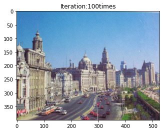
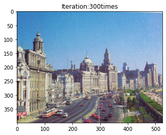
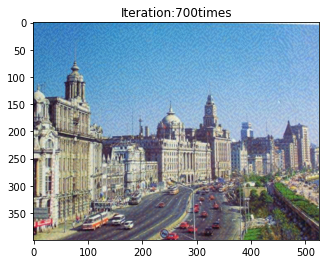
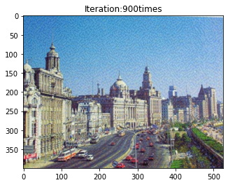
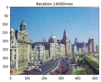
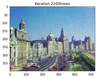
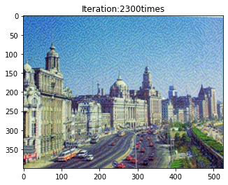
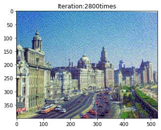
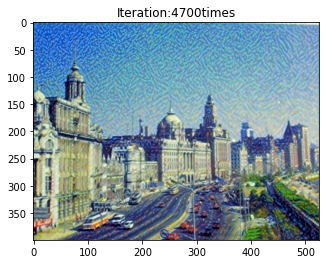
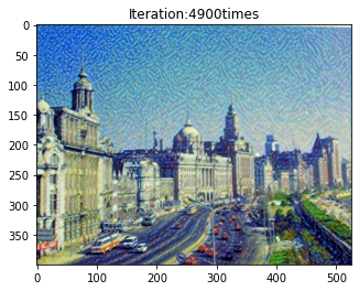
# Output per show_ The generated image after every iteration
if ii % show_every == 0:
print('Total loss:', total_loss.item())
print('Use time:', (time.time() - t0) / 3600, 'hour')
newim = im_convert(target)
plt.imshow(newim)
plt.title('Iteration:' + str(ii) + 'times')
plt.show()
# Save picture
result = Image.fromarray((newim * 255).astype(np.uint8))
result.save('./data/styletransfer/result/result' + str(ii) + '.png')
Total loss: 122845784.0
Use time: 0.09552362905608283 hour
Total loss: 94523616.0
Use time: 0.19464369164572823 hour

Total loss: 75496376.0
Use time: 0.2968603479862213 hour
Total loss: 62033356.0
Use time: 0.4009838284386529 hour

Total loss: 52134036.0
Use time: 0.5064849876695209 hour

Total loss: 44690424.0
Use time: 0.6129636422130796 hour

Total loss: 38979816.0
Use time: 0.7186389108498891 hour
Total loss: 34524896.0
Use time: 0.822829952902264 hour

Total loss: 30991986.0
Use time: 0.9157749527030521 hour
Total loss: 28144496.0
Use time: 1.0104362222221162 hour

Total loss: 25806564.0
Use time: 1.1048695998721652 hour

Total loss: 23855330.0
Use time: 1.2040331729915408 hour

Total loss: 22200796.0
Use time: 1.2968463142712912 hour

Total loss: 20776636.0
Use time: 1.3940133858389325 hour
Total loss: 19532510.0
Use time: 1.491570719215605 hour

Total loss: 18431378.0
Use time: 1.584603530433443 hour

Total loss: 17445626.0
Use time: 1.6766611027055316 hour

Total loss: 16553765.0
Use time: 1.77121149831348 hour

Total loss: 15739453.0
Use time: 1.8641047936677932 hour

Total loss: 14989285.0
Use time: 1.9569297609064313 hour

Total loss: 14294189.0
Use time: 2.053051912519667 hour

Total loss: 13646263.0
Use time: 2.15158909784423 hour
Total loss: 13039096.0
Use time: 2.245860044360161 hour
Total loss: 12466958.0
Use time: 2.3427789709303113 hour

Total loss: 11926141.0
Use time: 2.439336260954539 hour

Total loss: 11413008.0
Use time: 2.533568103114764 hour

Total loss: 10924717.0
Use time: 2.6285477293862236 hour

Total loss: 10458755.0
Use time: 2.7288781878021027 hour
Total loss: 10013593.0
Use time: 2.8237942422098583 hour

Total loss: 9587543.0
Use time: 2.9144839725229477 hour

Total loss: 9179240.0
Use time: 3.011672951777776 hour

Total loss: 8787736.0
Use time: 3.1060453993082047 hour

Total loss: 8411771.0
Use time: 3.18847301238113 hour

Total loss: 8050257.5
Use time: 3.2714244759745066 hour

Total loss: 7702339.5
Use time: 3.3536903029017977 hour

Total loss: 7367436.0
Use time: 3.436923085980945 hour

Total loss: 7045252.0
Use time: 3.5295680926243462 hour

Total loss: 6735090.0
Use time: 3.610985151529312 hour

Total loss: 6436338.0
Use time: 3.692777942617734 hour

Total loss: 6148604.0
Use time: 3.7746490195062425 hour

Total loss: 5871365.0
Use time: 3.8563965653710897 hour

Total loss: 5604487.0
Use time: 3.9382439964347418 hour

Total loss: 5347499.0
Use time: 4.020589534905222 hour

Total loss: 5100200.0
Use time: 4.10287761622005 hour

Total loss: 4862363.5
Use time: 4.193053228259086 hour

Total loss: 4633683.5
Use time: 4.289416976504856 hour

Total loss: 4414032.0
Use time: 4.39090823703342 hour
Total loss: 4203435.0
Use time: 4.492569035953945 hour

Total loss: 4001681.0
Use time: 4.573864739934604 hour
Total loss: 3808715.75
Use time: 4.657761905789375 hour

be careful:
The optimizer uses optim Adam ([target], LR = 0.0003), indicating that in the optimization, the final parameter to be optimized is the pixel value of the target image, and the weight and other parameters in the VGG network will not be optimized.
When calculating the content loss, it is necessary to extract the output of the specified layer, that is, use target_features ['conv4_2'] obtain the content representation of the target image and use content_features ['conv4_2'] obtain the content representation of the content image.
Since the loss of image style representation is represented by multiple layers, it is necessary to calculate the relevant Gram matrix and style loss layer by layer through circulation.
The sum of loss and loss is weighted.
In order to observe and preserve the results of image style in the migration process, the images are stored every 1000 1000 The results of 1000 iterations are visualized and saved to the specified file.
During the training, the loss of visual content, style and total loss are as follows:
plt.figure(figsize = (12, 4))
plt.subplot(1, 2 ,1)
plt.plot(total_loss_all, 'r', label = 'total_loss')
plt.legend()
plt.title('Total Loss')
plt.subplot(1, 2, 2)
plt.plot(content_loss_all, 'g-', label = 'content_loss')
plt.plot(style_loss_all, 'b-', label = 'style_loss')
plt.legend()
plt.title('Content and Style Loss')
plt.show()
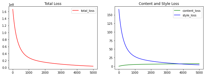
The initialization of the target image is the content image, so in the training process, the content loss gradually increases and the style loss gradually decreases, indicating that the style of the target image is more obvious.