preface

The reason why I want to send this is that I'm angry when I think about it. Last time, because of the change in the number of cases in the database (the change in the inclusion and exclusion criteria of cases), I made statistical analysis for many times, repeatedly modified my third-line table, and was scolded by my boss for filling in the wrong data several times. I'm angry when I think of it, and then I learned the function table1 angrily. It's very easy to make the third-line table next time. I'm happy.

I will write this part of the third line table in 2-3 parts. Today I write the first part: mainly to optimize the contents of the third line table. Next time, we will mainly talk about adding columns such as P value and chi square value.

The three line table directly drawn in Table 1 outputs all the mean and median values for continuous data without judging the normality of the data.
The problem solved in this paper: for the measurement data, it is divided into positive attitude distribution and non normal distribution, which are expressed by mean(± sd) and median(min, max) respectively. In this way, we also omit the steps of normality test.

Let's see the effect first. Pay attention to which line of age and normality data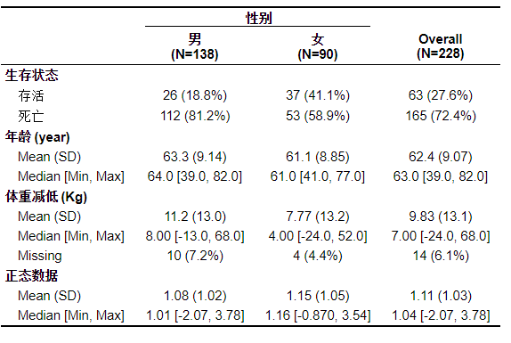

If you just want to use it, skip directly to the final code summary part, and the content in the middle may be more suitable for comrades who break the casserole and ask to the end.

Tip: I won't repeat the title, header and footnote added to table1, because this part is not important to us. Want to know how to make good use of the browser

1, table1

Let's first understand the process of drawing a three line table of this function, which can be understood in this way. Each time a cross grid is drawn, as shown in the red circle in the above figure, the function will pass in the survival status data of all men and women in the data frame, and then take the calculation frequency. Some of the following processes may be obscure. You are welcome to ask questions or send private letters in the comment area.

2, Simple production

1. General process (using formula form)

In fact, table1 can be put into either formula format (simple) or strata and labels format (flexible).

The code is as follows (example):

rm(list = ls())
library(table1)
library(survival)
options(stringsAsFactors = F)
a <- lung
str(a)

#Set the factor. It should be noted that the classification variable must be set to factor or string format, otherwise it will be calculated as a value. Here, gender and survival status are classification variables.
a$sex <- factor(a$sex,levels = c(1,2),labels = c('male','female'))
a$status <- factor(a$status,levels = c(1,2),labels = c("survival","death"))

#It can be verified that age is non normal data. This p > 0.1 indicates that it is normal, and vice versa.
shapiro.test(a$age)$p.value

#In order to verify whether different formats can be output according to the normality of data, a group of normal data is added here.
a$normdata <- rnorm(nrow(a),1,1)

#Set the missing value to see if the function can recognize the missing data
a$age[3] <- NA

#Set the unit so that the unit can be displayed in the row name, as shown in (years, Kg) in the figure
units(a$age) <- 'year'
units(a$wt.loss) <- 'Kg'

#Set the label. The label here is the row name. Otherwise, the row names of the three line table will be displayed as status, age, and so on
label(a$status) <- "Survival state"
label(a$age) <- "Age"
label(a$wt.loss) <- "Weight loss"
label(a$sex) <- "Gender"
label(a$normdata) <- "Normal data"
table1(~status+age+wt.loss+normdata|sex,data = a)

2. Problems found

After running the code, the three line table we want does appear, but did you find it? Whether our data is normal or not, it will output the mean (standard deviation) and median (extreme value). This is not what we want. In order to delete, we have to re test the normality and delete it line by line. Obviously, this is not our original intention to learn R language.

3. Clues

Leaving aside this question, let's learn how to change this three-line table first?
Take a look at the help document. I have explored it for you. The data in the table is passed through the render parameter.
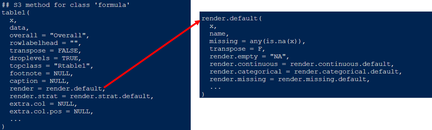Render points to a render Default function, render Default contains the transfer of continuous variables, classified variables and null values. It is in the form of functions. Call up the code of these two functions and have a look.

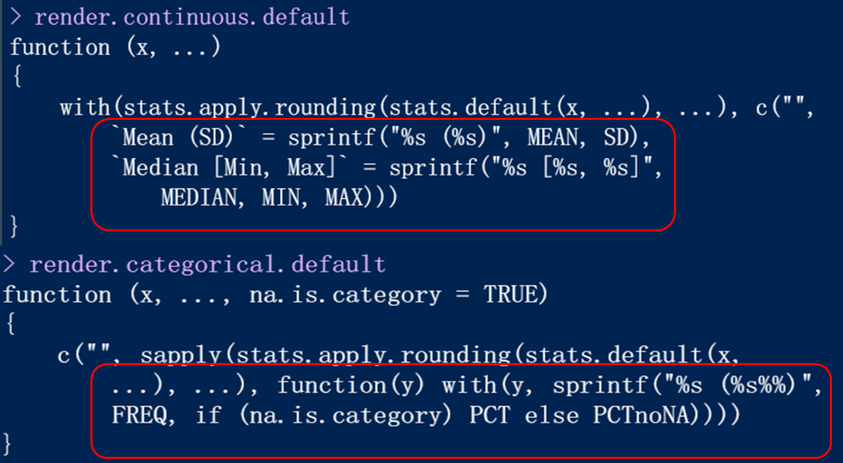
From the function, you can find the manifestations of classified variables and numerical variables (marked by red box).

Here I rewrite the render function and render continuous. The default function preliminarily realizes the selective output of the function according to the normal test.

The code is as follows (example):

rewrite render.default function
rd <- function(x, name, ...){
#The parameters x and name passed in here
#For example, when drawing the grid of men's age (all the examples below are this), x is: the gender of the data is all the age data of men. Name is age, so a[[name]] here is used to extract age data in data a (both men and women)
  y <- a[[name]]
#Judge whether there is a null value in the age data. If it is null, we need to add the missing line
  m = any(is.na(y))
#It is processed separately according to whether the incoming data is a numerical value
  if (is.numeric(y)) {
#Judge whether it is normal, and pass the judgment result to my render. In the cont function
    normt=(shapiro.test(y)$p.value>0.1)+2
    my.render.cont(x,n=normt,m=m,...)
  }else{
#Because we don't need to deal with classification variables, we just call the default function here
    render.default(x=x, name=name, ...)
    }
  }
  
#Override render continuous. Default function.
my.render.cont <- function (x,n,m, ...) {
#x has the same meaning as in the above function. n is the result of judging whether it is normal and m is the result of judging whether it is null
  a=with(stats.apply.rounding(stats.default(x, ...), ...), c("", 
                                                           `Mean (±SD)` = sprintf("%s (±%s)", MEAN, SD),
                                                           `Median (Min, Max)` = sprintf("%s (%s, %s)", MEDIAN, MIN, MAX)
                                                           ))[-n] #Determine the output mean or median according to the normal judgment result
  if (m) {
    a <- c(a,with(stats.apply.rounding(stats.default(is.na(x), ...), ...)$Yes,
                  c(`Missing` = sprintf("%s (%s%%)", FREQ, PCT))))
                  #Here, the missing line is output according to whether there is a null value
  }
  a
}

###The last step is to run our function of drawing three line table, render parameter and render Replace the continuous parameter with the function we override.
table1(~status+age+wt.loss+normdata|sex,data = a,render = rd,render.continuous=my.render.cont)

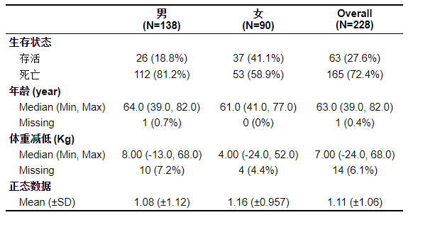
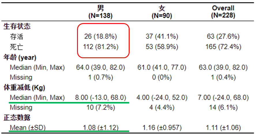
The graph is perfect. It can be found that the presentation form of normal data and non normal data is different.

4. Code summary

Finally, of course, the code should be summarized for your convenience

rm(list = ls())
library(survival)
library(survminer)
library(table1)
options(stringsAsFactors = F)
#Rewrite function
rd <- function(x, name, ...){
  y <- a[[name]]
  m = any(is.na(y))
  if (is.numeric(y)) {
    normt=(shapiro.test(y)$p.value>0.1)+2
    my.render.cont(x,n=normt,m=m,...)
  }else{
    render.default(x=x, name=name, ...)
    }
  }

#Override continuous variable handler
my.render.cont <- function (x,n,m, ...) {
  
  a=with(stats.apply.rounding(stats.default(x, ...), ...), c("", 
                                                             `Mean (±SD)` = sprintf("%s (±%s)", MEAN, SD),
                                                             `Median (Min, Max)` = sprintf("%s (%s, %s)", MEDIAN, MIN, MAX)
  ))[-n]
  if (m) {
    a <- c(a,with(stats.apply.rounding(stats.default(is.na(x), ...), ...)$Yes,
                  c(`Missing` = sprintf("%s (%s%%)", FREQ, PCT))))
  }
  a
}
#########################Dividing line#############################################
####The above part can be reused without change. The following part needs you to change your own data and change some contents
############################################################################
a <- lung
str(a)

#Setting factors, taking age, gender, weight loss and status as examples
a$sex <- factor(a$sex,levels = c(1,2),labels = c('male','female'))
a$status <- factor(a$status,levels = c(1,2),labels = c("survival","death"))
a$normdata <- rnorm(nrow(a),1,1)
a$age[3] <- NA

#Set unit
units(a$age) <- 'year'
units(a$wt.loss) <- 'Kg'

#Set label
label(a$status) <- "Survival state"
label(a$age) <- "Age"
label(a$wt.loss) <- "Weight loss"
label(a$sex) <- "Gender"
label(a$normdata) <- "Normal data"
table1(~status+age+wt.loss+normdata|sex,data = a)
table1(~status+age+wt.loss+normdata|sex,data = a,render = rd,render.continuous=my.render.cont)
##Which one do you prefer?

summary

In fact, I've seen this function before, but at that time, I just had a playful attitude and learned a little knowledge. This time, I really want to learn from the pain and want to solve it.
Notice: the next article is to add the p value of chi square test and t-test
I am still a beginner. If I make mistakes, I welcome criticism and correction, and accept your suggestions with an open mind.