animalcules is an R software package used to provide users with an easy-to-use interactive microbiome analysis framework using the latest data analysis, visualization methods and machine learning models. It can be used as a stand-alone software package, or users can explore their data with the accompanying interactive R Shiny application.
Traditional microbiome analysis, such as α/β Diversity and differential abundance analysis have been strengthened, while new methods, such as biomarker recognition, have been introduced by animal molecules. animalcules generates powerful interactive and dynamic numbers that enable users to better understand their data and discover new insights.
introduce
The animalcules * package focuses on the unified framework of microbiome data, and then packages the current popular analysis methods and means. The author says that the traditional alpha and beta diversity has been too rampant, so it is more powerful to introduce the biomarker analysis method into the * animalcules * package, and then use interactive charts to analyze and understand the data. We must note that this kind of framework uses S4 class objects, otherwise it will not be so convenient.
The following tutorials mainly refer to the software help manual. See the original text for details: https://bioconductor.org/packages/release/bioc/vignettes/animalcules/inst/doc/animalcules.html
R package installation
There are many software dependencies. For example, some Packages that fail to be installed automatically also need to be installed manually in the Packages management center in RStudio.
#--Install the R package used by BiocManager to install Bioconductor
if (!requireNamespace("BiocManager", quietly=TRUE))
  install.packages("BiocManager")
#--BiocManager installs the animalcules package in Bioconductor
if (!requireNamespace("animalcules", quietly=TRUE))
  BiocManager::install("compbiomed/animalcules")

## Install github version
if (!requireNamespace("devtools", quietly=TRUE))
   install.packages("devtools")
if (!requireNamespace("animalcules", quietly=TRUE))
  devtools::install_github("compbiomed/animalcules")
#The following shows that the built-in phyloseq object data set is used when constructing the MultiAssayExperiment object
if (!requireNamespace("ggClusterNet", quietly=TRUE))
  devtools::install_github("taowenmicro/ggClusterNet")

#--Load R package
library(animalcules)
library(SummarizedExperiment)
library(MultiAssayExperiment)
data_dir = system.file("extdata/MAE.rds", package = "animalcules")
MAE = readRDS(data_dir)
Necessary knowledge about data format
In a word, if you want more convenience, you need more encapsulation, consistent format and unified format.
The default data analysis MAE of the author: in fact, the core is summarized experiment data, and multiple summarized experiments are MultiAssayExperiment. This is a good framework for multi omics data integration. Let's briefly introduce it
Multiomics data processing ideas
Omics experiments are becoming more and more common, which increases the complexity of experimental design, data integration and analysis. R and Bioconductor provide a general framework for statistical analysis and visualization, and provide special data classes for various high-throughput data types, but they lack the method of integrated analysis of multiomics experiments.
MultiAssayExperiment
The integrated R package of multiomics experiment, MultiAssayExperiment, provides consistent representation, storage and operation for a variety of genomic data.
MultiAssayExperiment( https://bioconductor.org/packages/MultiAssayExperiment )An object-oriented S4 class object is introduced, and a general data structure for representing multiomics experiments is defined. It has three key components:
(i)colData, a "primary" data set containing characteristics at the patient or cell line level, such as pathology and histology;
(ii)ExperimentList, the main data storage object, can include multiple groups of data.
(iii)sampleMap, a map file used to link all data.
-
(1) Constructors and related validity checks simplify the creation of MultiAssayExperiment objects while allowing flexibility to represent complex experiments.
-
(2) Subset operations for data selection are allowed.
The MultiAssayExperiment core data is based on SummarizedExperiment and supports heterogeneous multiomics data at the same time. MultiAssayExperiment classes and methods provide a flexible framework for integrating and analyzing complementary analysis of overlapping samples. It integrates any data class that supports basic subset and dimension names, so many data classes are supported by default without additional adjustment.
#-Some basic operations on A MultiAssayExperiment object
#Assessments section
# assays(MAE)# Extract the data matrix part of the file, which is a list, so the extraction of each matrix needs to continue
#--What's the use of extracting the first matrix? Similar to multi omics data, it is easier to operate.
# assays(MAE)[[1]]# The second object is similar
# assays(MAE)[[2]]
#--colData, that is, the annotation information for the column names of the data matrix, is similar to the map file in the phyloseq object
colData(MAE)

#--Check the number of sub objects, which are s4 objects and can be extracted separately

#--Extract each part of data for a single S4 object
microbe <- MAE[["MicrobeGenetics"]]
otu_table <- as.data.frame(SummarizedExperiment::assays(microbe))
tax_table <- as.data.frame(SummarizedExperiment::rowData(microbe))
map <- as.data.frame(SummarizedExperiment::colData(microbe))
Constructing a MultiAssayExperiment object
Building MultiAssayExperiment objects using phyloseq objects
As for how to construct phyloseq files, You can click to view . If you want to learn specifically what a phyloseq object is, Can click
# How to build this MAE object?

#--Get the phyloserq object and extract the necessary data information
library(ggClusterNet)
library(phyloseq)
ps
otu = as.data.frame(t(vegan_otu(ps)))
head(otu)
tax = as.data.frame((vegan_tax(ps)))
head(tax)
map = sample_data(ps)
head(map)
#--First, construct the SummarizedExperiment object, which is relatively simple and similar to the phyloseq object
micro <- SummarizedExperiment(assays=list(counts=as.matrix(otu)),
                              colData=map,
                              rowData=tax)
# Encapsulate the SummarizedExperiment object as an ExperimentList
mlist <- ExperimentList()
mlist[[1]] = micro
names(mlist) = "MicrobeGenetics"# Note that it must be named, otherwise each partial data group cannot be distinguished
# Constructing record files between different data groups
gistmap <- data.frame(
  primary = row.names(map),
  colname = row.names(map),
  stringsAsFactors = FALSE)
maplistowe <- list(MicrobeGenetics = gistmap)
sampMapowe <- listToMap(maplistowe)

# The colData file is a grouping file, and the data frame is enough. In this case, there is only one microbiome data, so you can directly use the map file.
#-The MultiAssayExperiment file is built directly below
mae <- MultiAssayExperiment(experiments = mlist, colData = map,
                            sampleMap = sampMapowe)
Run Shiny app

Here we have prepared our own example file to ensure that this tool can be turned into an ordinary tool for everyone to use as much as possible.
run_animalcules()
### Basic statistics
The next part, I will run at the same time Shiny Compare with the official code tutorial, but it will not dig deeply. It will only help you complete the official tutorial and put forward some suggestions. Second, although we also build MAE However, due to some minor defects in the author's code, the official data is used for demonstration.
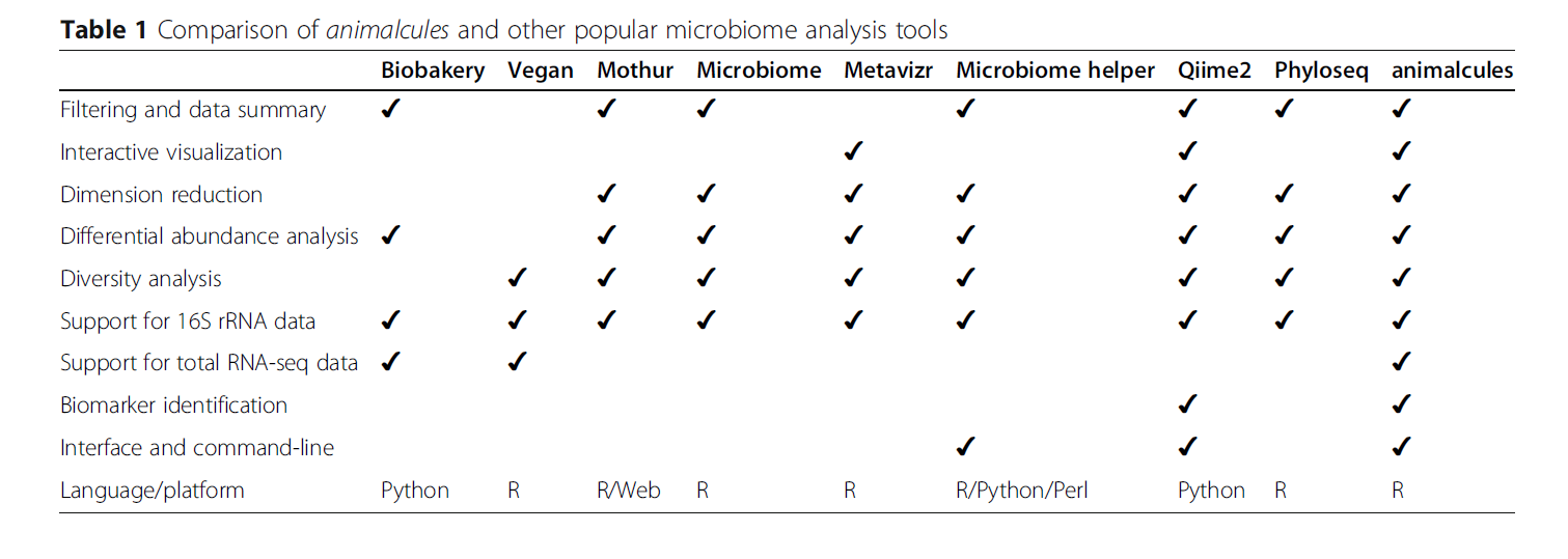
This part is used for statistics in each sample OTU And do visualization in two ways: frequency curve and box line+Scatter diagram; If used shiny Program, you can directly display the form.

In addition, it can be combined according to the level of microbial classification OTU Data:

- samples_discard : Samples to be removed id
```{R}
# ?filter_summary_pie_box
p <- filter_summary_pie_box(MAE,
samples_discard = c("subject_2", "subject_4"),
filter_type = "By Metadata",
sample_condition = "AGE")
p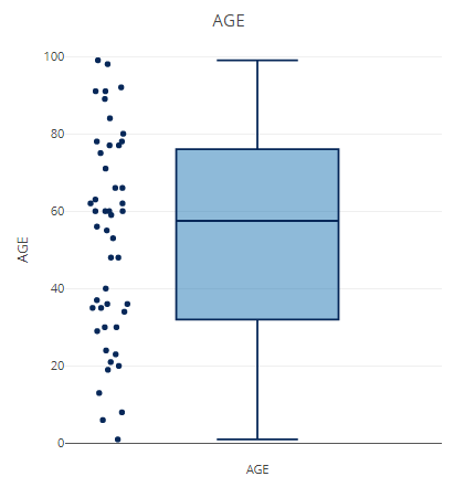
Change the group and make statistics again.
p <- filter_summary_bar_density(MAE,
                                samples_discard = c("subject_2", "subject_4"),
                                filter_type = "By Metadata",
                                sample_condition = "SEX")
p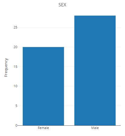
#--Extract the subset and extract the map file
microbe <- MAE[['MicrobeGenetics']]
samples <- as.data.frame(colData(microbe))
result <- filter_categorize(samples,
                            sample_condition="AGE",
                            new_label="AGE_GROUP",
                            bin_breaks=c(0,55,75,100),
                            bin_labels=c('Young','Adult',"Elderly"))
head(result$sam_table)
result$plot.binned
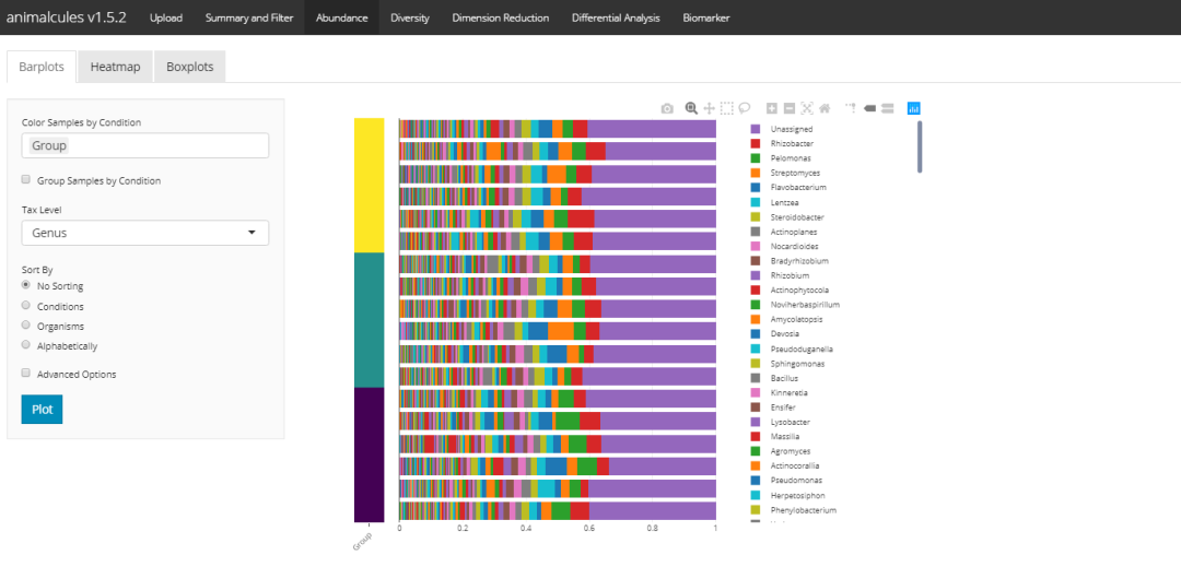
Abundance display - stacked histogram
Via tax_level select a classification level through sample_conditions select the group label you want to add. It is worth noting that the stacked histogram can be sorted here through order_ Organizations to specify the default abundance from high to low. From the source code point of view, it is realized by changing the factor, so the first microorganism in the legend is also the sorted microorganism.
p <- relabu_barplot(MAE,
                    tax_level="family",
                    order_organisms=c('Retroviridae'),
                    sort_by="organisms",
                    sample_conditions=c('SEX', 'AGE'),
                    show_legend=TRUE)
p
shiny version:
Abundance heat map
p <- relabu_heatmap(MAE,
                   tax_level="genus",
                   sort_by="conditions",
                   sample_conditions=c("SEX", "AGE"))
p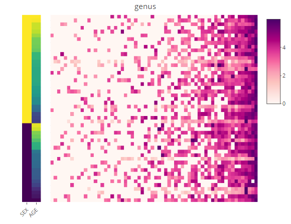
shiny version:

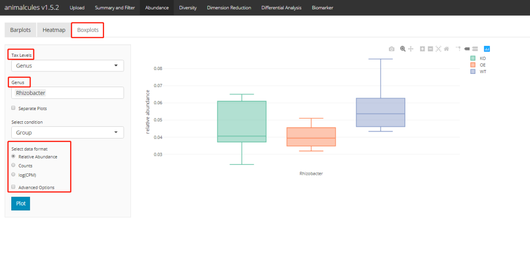
Abundance box plot
p <- relabu_boxplot(MAE,
                    tax_level="genus",
                    organisms=c("Escherichia", "Actinomyces"),
                    condition="SEX",
                    datatype="logcpm")
p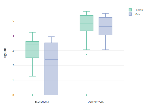
shiny version:
Alpha diversity
There are only four diversity indicators. Then it is displayed through box line + scatter diagram.
alpha_div_boxplot(MAE = MAE,
                  tax_level = "genus",
                  condition = "DISEASE",
                  alpha_metric = "shannon")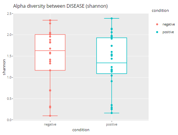
The diversity was statistically tested. Here, three methods are available: "Wilcoxon rank sum test", "T-test" and "Kruskal Wallis".
# ?do_alpha_div_test
do_alpha_div_test(MAE = MAE,
                  tax_level = "genus",
                  condition = "DISEASE",
                  alpha_metric = "shannon",
                  alpha_stat = "T-test")
shiny version:

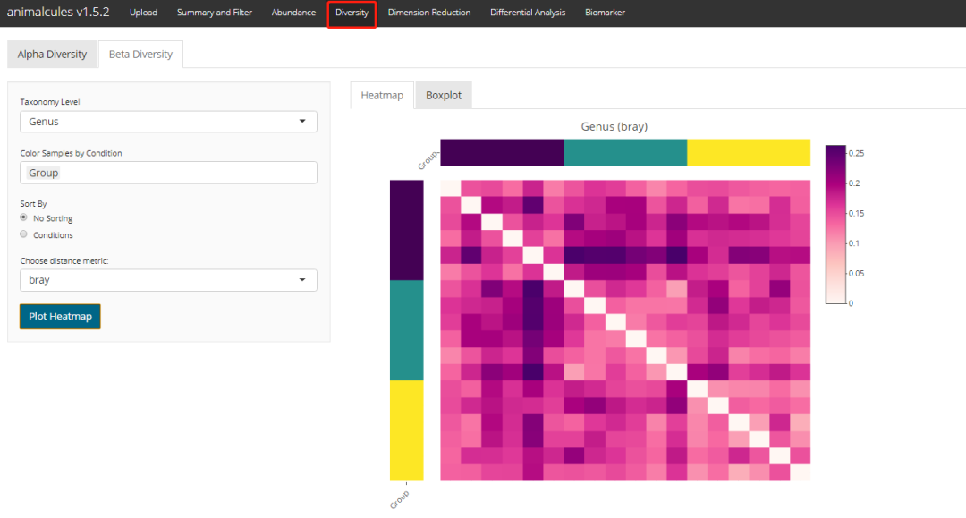
Beta diversity clustering distance heat map
diversity_beta_heatmap(MAE = MAE,
                       tax_level = 'genus',
                       input_beta_method = "bray",
                       input_bdhm_select_conditions = 'DISEASE',
                       input_bdhm_sort_by = 'condition')
Beta diversity - inter group distance box diagram
Secondly, it is displayed through the box diagram of the distance between groups and the distance between groups
diversity_beta_boxplot(MAE = MAE,
                       tax_level = 'genus',
                       input_beta_method = "bray",
                       input_select_beta_condition = 'DISEASE')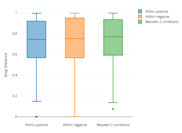
Another is statistical test. There are three methods to choose from: permanova, Kruskal Wallis and Wilcoxon test.
However, there are only two distances to choose from, and the second is that pairwise comparison cannot be realized.
# ?diversity_beta_test
diversity_beta_test(MAE = MAE,
                    tax_level = 'genus',
                    input_beta_method = "bray",
                    input_select_beta_condition =  'DISEASE',
                    input_select_beta_stat_method = 'PERMANOVA',
                    input_num_permutation_permanova = 999)
shiny version:
shiny Version (error):

sort
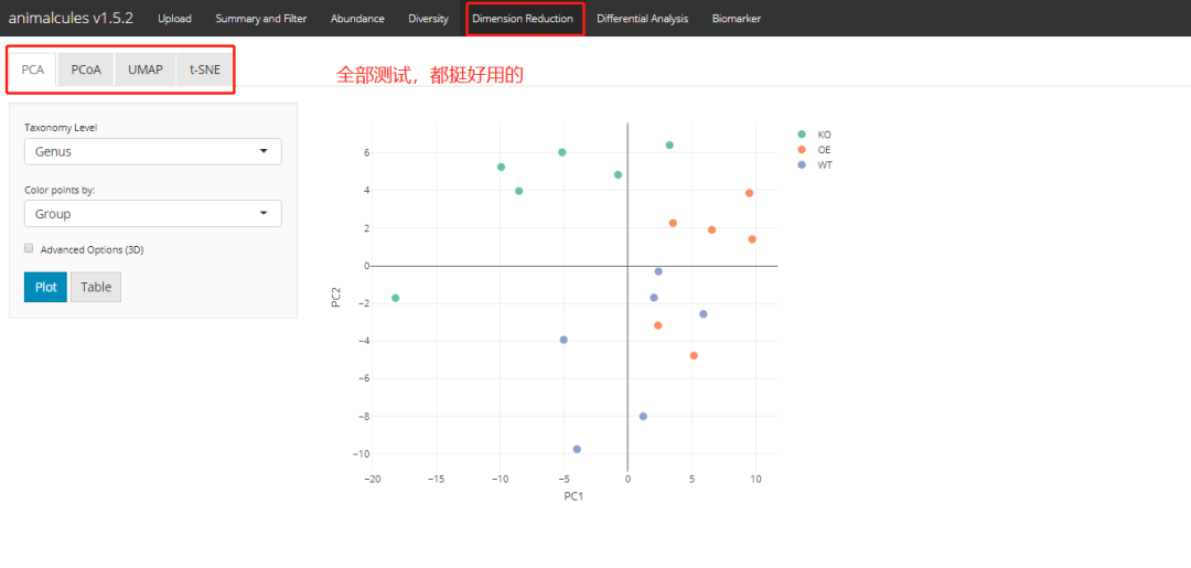
PCA
result <- dimred_pca(MAE,
                     tax_level="genus",
                     color="AGE",
                     shape="DISEASE",
                     pcx=1,
                     pcy=2,
                     datatype="logcpm")
result$plot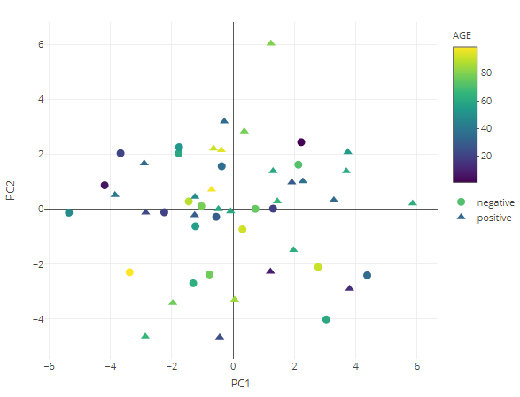
PCoA
result <- dimred_pcoa(MAE,
                      tax_level="genus",
                      color="AGE",
                      shape="DISEASE",
                      axx=1,
                      axy=2,
                      method="bray")
result$plot
result$plot

UMAP
result <- dimred_umap(MAE,
                      tax_level="genus",
                      color="AGE",
                      shape="DISEASE",
                      cx=1,
                      cy=2,
                      n_neighbors=15,
                      metric="euclidean",
                      datatype="logcpm")
result$plot
t-SNE
In addition to two-dimensional graphic display, it can also display three-dimensional graphics.
result <- dimred_tsne(MAE,
                      tax_level="phylum",
                      color="AGE",
                      shape="GROUP",
                      k="3D",
                      initial_dims=30,
                      perplexity=10,
                      datatype="logcpm")
result$plot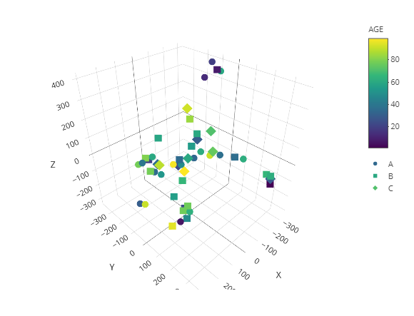
shiny version:
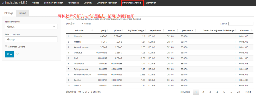
Difference analysis
p <- differential_abundance(MAE,
                            tax_level="phylum",
                            input_da_condition=c("DISEASE"),
                            min_num_filter = 2,
                            input_da_padj_cutoff = 0.5)
p
shiny version:
Biomarker analysis
There are two optional methods: "logistic regression" and "random forest".
# ?find_biomarker
p <- find_biomarker(MAE,
                    tax_level = "genus",
                    input_select_target_biomarker = c("SEX"),
                    nfolds = 3,
                    nrepeats = 3,
                    seed = 99,
                    percent_top_biomarker = 0.2,
                    model_name = "logistic regression")
p$biomarker
Visualize important variables.
# importance plot
p$importance_plot

ROC curve accuracy evaluation. Note that ROC curve can only operate on binary variables.
p$roc_plot
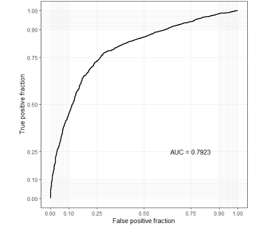
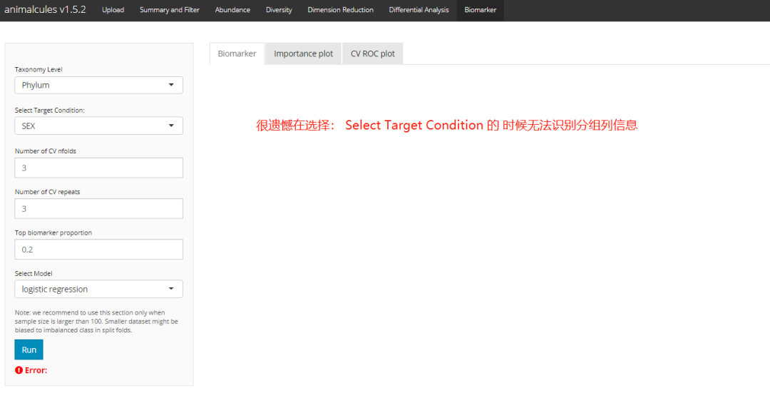
shiny Version (error):
Operating environment
sessionInfo()
R version 4.1.0 (2021-05-18)
Platform: x86_64-w64-mingw32/x64 (64-bit)
Running under: Windows 10 x64 (build 19042)

Matrix products: default

locale:
[1] LC_COLLATE=Chinese (Simplified)_China.936
[2] LC_CTYPE=Chinese (Simplified)_China.936
[3] LC_MONETARY=Chinese (Simplified)_China.936
[4] LC_NUMERIC=C
[5] LC_TIME=Chinese (Simplified)_China.936

attached base packages:
[1] parallel  stats4    stats     graphics  grDevices utils     datasets
[8] methods   base

other attached packages:
 [1] caret_6.0-88                biomformat_1.20.0
 [3] magrittr_2.0.1              dplyr_1.0.6
 [5] vegan_2.5-7                 lattice_0.20-44
 [7] permute_0.9-5               plotly_4.9.3
 [9] ggplot2_3.3.3               shinyjs_2.0.0
[11] shiny_1.6.0                 phyloseq_1.36.0
[13] ggClusterNet_0.1.0          MultiAssayExperiment_1.18.0
[15] SummarizedExperiment_1.22.0 Biobase_2.52.0
[17] GenomicRanges_1.44.0        GenomeInfoDb_1.28.0
[19] IRanges_2.26.0              S4Vectors_0.30.0
[21] BiocGenerics_0.38.0         MatrixGenerics_1.4.0
[23] matrixStats_0.58.0          animalcules_1.9.1

loaded via a namespace (and not attached):
  [1] utf8_1.2.1             reticulate_1.20        tidyselect_1.1.1
  [4] RSQLite_2.2.7          AnnotationDbi_1.54.0   htmlwidgets_1.5.3
  [7] ranger_0.12.1          grid_4.1.0             BiocParallel_1.26.0
 [10] covr_3.5.1             pROC_1.17.0.1          devtools_2.4.2
 [13] munsell_0.5.0          codetools_0.2-18       DT_0.18
 [16] umap_0.2.7.0           rentrez_1.2.3          withr_2.4.2
 [19] colorspace_2.0-1       knitr_1.33             rstudioapi_0.13
 [22] labeling_0.4.2         GenomeInfoDbData_1.2.6 plotROC_2.2.1
 [25] bit64_4.0.5            farver_2.1.0           rhdf5_2.36.0
 [28] rprojroot_2.0.2        vctrs_0.3.8            generics_0.1.0
 [31] ipred_0.9-11           xfun_0.23              R6_2.5.0
 [34] locfit_1.5-9.4         rex_1.2.0              bitops_1.0-7
 [37] rhdf5filters_1.4.0     cachem_1.0.5           DelayedArray_0.18.0
 [40] assertthat_0.2.1       promises_1.2.0.1       scales_1.1.1
 [43] nnet_7.3-16            gtable_0.3.0           processx_3.5.2
 [46] timeDate_3043.102      rlang_0.4.11           genefilter_1.74.0
 [49] splines_4.1.0          lazyeval_0.2.2         ModelMetrics_1.2.2.2
 [52] GUniFrac_1.2           BiocManager_1.30.15    yaml_2.2.1
 [55] reshape2_1.4.4         crosstalk_1.1.1        httpuv_1.6.1
 [58] tools_4.1.0            lava_1.6.9             usethis_2.0.1
 [61] ellipsis_0.3.2         jquerylib_0.1.4        RColorBrewer_1.1-2
 [64] proxy_0.4-26           sessioninfo_1.1.1      Rcpp_1.0.6
 [67] plyr_1.8.6             progress_1.2.2         zlibbioc_1.38.0
 [70] purrr_0.3.4            RCurl_1.98-1.3         ps_1.6.0
 [73] prettyunits_1.1.1      rpart_4.1-15           openssl_1.4.4
 [76] cluster_2.1.2          fs_1.5.0               data.table_1.14.0
 [79] RSpectra_0.16-0        pkgload_1.2.1          hms_1.1.0
 [82] mime_0.10              evaluate_0.14          xtable_1.8-4
 [85] XML_3.99-0.6           shape_1.4.6            testthat_3.0.2
 [88] compiler_4.1.0         tibble_3.1.2           crayon_1.4.1
 [91] htmltools_0.5.1.1      mgcv_1.8-35            later_1.2.0
 [94] tidyr_1.1.3            geneplotter_1.70.0     lubridate_1.7.10
 [97] DBI_1.1.1              MASS_7.3-54            Matrix_1.3-3
[100] ade4_1.7-16            cli_2.5.0              gower_0.2.2
[103] igraph_1.2.6           forcats_0.5.1          pkgconfig_2.0.3
[106] recipes_0.1.16         foreach_1.5.1          annotate_1.70.0
[109] bslib_0.2.5.1          multtest_2.48.0        XVector_0.32.0
[112] prodlim_2019.11.13     stringr_1.4.0          callr_3.7.0
[115] digest_0.6.27          tsne_0.1-3             Biostrings_2.60.0
[118] rmarkdown_2.8          curl_4.3.1             lifecycle_1.0.0
[121] nlme_3.1-152           jsonlite_1.7.2         Rhdf5lib_1.14.0
[124] desc_1.3.0             viridisLite_0.4.0      askpass_1.1
[127] limma_3.48.0           fansi_0.5.0            pillar_1.6.1
[130] KEGGREST_1.32.0        fastmap_1.1.0          httr_1.4.2
[133] pkgbuild_1.2.0         survival_3.2-11        glue_1.4.2
[136] remotes_2.4.0          png_0.1-7              iterators_1.0.13
[139] glmnet_4.1-1           bit_4.0.4              class_7.3-19
[142] stringi_1.6.2          sass_0.4.0             blob_1.2.1
[145] DESeq2_1.32.0          memoise_2.0.0          e1071_1.7-7
[148] ape_5.5
Reference
-
https://bioconductor.org/packages/release/bioc/vignettes/animalcules/inst/doc/animalcules.html
reference:
Interactive microbiome analysis toolkit • animalcules (compbiomed.github.io)
Zhao, Yue, Anthony Federico, Tyler Faits, Solaiappan Manimaran, Daniel Segrè, Stefano Monti, and W. Evan Johnson. "animalcules: interactive microbiome analytics and visualization in R." Microbiome 9, no. 1 (2021): 1-16.