[RNN architecture analysis] LSTM model

preface

Understand the internal structure and calculation formula of LSTM
Master the use of LSTM tools in pytoch
Understand the advantages and disadvantages of LSTM

LSTM (long short term memory), also known as long short term memory structure, is a variant of traditional RNN. Compared with classical RNN, it can effectively capture the semantic association between long sequences and alleviate the phenomenon of gradient disappearance or explosion. At the same time, the structure of LSTM is more complex, and its core structure can be divided into four parts:

Forgetting gate
Input gate
Cell state
Output gate

1. Internal structure diagram of LSTM

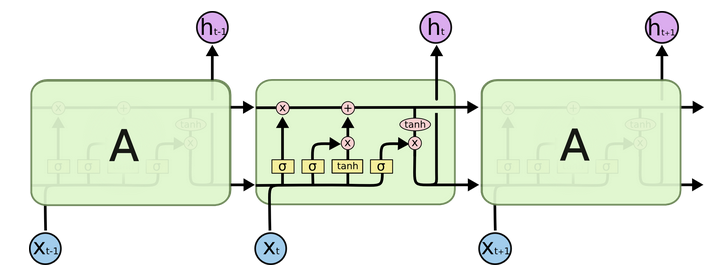
Structure explanation diagram:

Structural drawing and calculation formula of forgetting door:

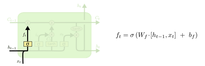
Structural analysis of door:

It is very similar to the internal structure calculation of traditional RNN. Firstly, the current time step input x(t) is spliced with the implicit state h(t-1) of the previous time step to obtain [x(t), h(t-1)], and then transformed through a full connection layer. Finally, f(t) is activated through the sigmoid function to obtain f(t). We can regard f(t) as the door value, such as the size of a door opening and closing, The gate value will act on the tensor passing through the gate, and the forgetting gate value will act on the cell state of the upper layer, representing how much information has been forgotten in the past. Because the forgetting gate value is calculated by x(t), h(t-1), the whole formula means that according to the current time step input and the implicit state h(t-1) of the previous time step To determine how much past information carried by the cell state of the upper layer is forgotten

Process demonstration of forgetting the internal structure of the door:

Function of activation function sigmiod:

To help adjust the value flowing through the network, the sigmoid function compresses the value between 0 and 1

Enter the structural drawing and calculation formula of the door:

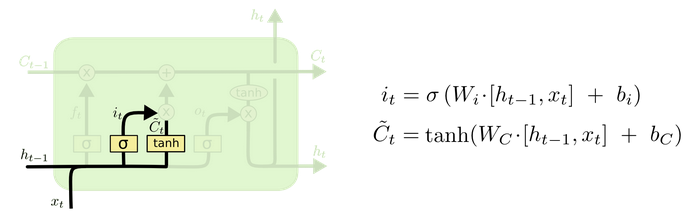
Input door structure analysis:

We can see that there are two formulas for calculating the input gate. The first is the formula for generating the input gate value, which is almost the same as the forgetting gate formula, except for the target they will act on later. This formula means that how much input information needs to be filtered. The second formula of the input gate is the same as the internal structure calculation of the traditional RNN. For LSTM, It gets the current cell state, not the implicit state like the classical RNN

Input door internal structure process demonstration:

Cell status update diagram and calculation formula:

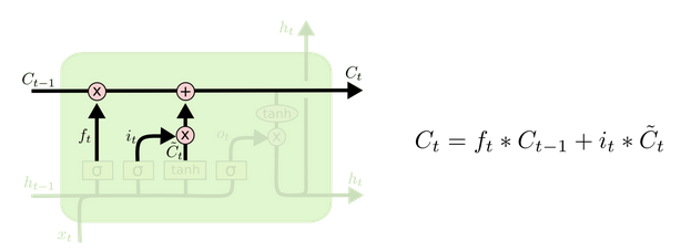
Cell status update analysis:

The structure and calculation formula of cell renewal are very easy to understand. There is no full connection layer here. Just multiply the just obtained forgetting gate value by the C(t-1) obtained in the previous time step, plus the result of multiplying the input gate value by the non updated C(t) obtained in the current time step. Finally, the updated C(t) is obtained As part of the next time step input, the whole cell state update process is the application of forgetting gate and input gate

Demonstration of cell status update process:

Structure diagram and calculation formula of output door: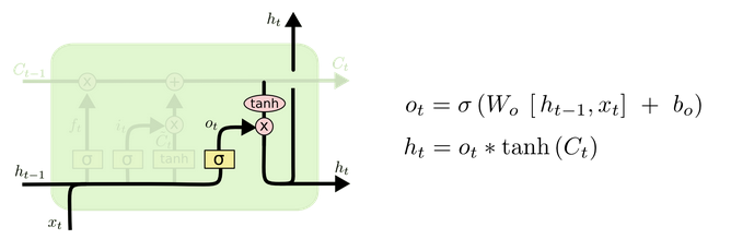

Structural analysis of output gate:

There are also two formulas for the output gate part. The first is to calculate the gate value of the output gate, which is the same as that of the forgetting gate and the input gate. The second is to use this gate value to generate the implicit state h(t), which will act on the updated cell State C(t) and activate tanh, and finally obtain h(t) as part of the input of the next time step. The whole process of the output gate, Is to produce the implicit state h(t)

Internal structure process demonstration of output door:

2. Bi LSTM introduction

What is bi LSTM?

Bi LSTM is bidirectional LSTM. It does not change any internal structure of the LSTM itself, but applies the LSTM twice in different directions, and then splices the LSTM results obtained twice as the final output

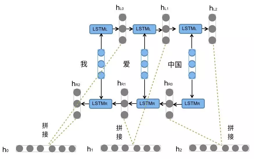
Bi LSTM structure analysis:

We can see that the sentence "I love China" or the input sequence in the figure is processed from left to right and from right to left, and the resulting tensors are spliced as the final output. * * this structure can capture some specific pre or post features in language grammar and enhance semantic correlation, * * but the model parameters and computational complexity are also doubled, It is generally necessary to evaluate the corpus and computing resources to decide whether to use the structure

3. Implementation of LSTM code

Use of LSTM tools in Pytorch:

Location: in torch.nn toolkit, it can be called through torch.nn.LSTM

nn.LSTM class initialization main parameter explanation:

input_size: enter the size of characteristic dimension in tensor x
hidden_size: the size of characteristic dimension in hidden layer tensor h
num_layers: number of hidden layers
Bidirectional: select whether to use bidirectional LSTM. If True, use; Not used by default

nn.LSTM class instantiation object main parameter interpretation:

Input: input tensor x
h0: initialized hidden layer tensor h
c0: initialized cell state tensor c

nn.LSTM usage example:

# Define the meaning of LSTM parameters: (input_size, hidden_size, num_layers)
# Define the parameter meaning of input tensor: (sequence_length, batch_size, input_size)
# Define the parameter meaning of hidden layer initial tensor and cell initial state tensor:
# (num_layers * num_directions, batch_size, hidden_size)

>>> import torch.nn as nn
>>> import torch
>>> rnn = nn.LSTM(5, 6, 2)
>>> input = torch.randn(1, 3, 5)
>>> h0 = torch.randn(2, 3, 6)
>>> c0 = torch.randn(2, 3, 6)
>>> output, (hn, cn) = rnn(input, (h0, c0))
>>> output
tensor([[[ 0.0447, -0.0335,  0.1454,  0.0438,  0.0865,  0.0416],
         [ 0.0105,  0.1923,  0.5507, -0.1742,  0.1569, -0.0548],
         [-0.1186,  0.1835, -0.0022, -0.1388, -0.0877, -0.4007]]],
       grad_fn=<StackBackward>)
>>> hn
tensor([[[ 0.4647, -0.2364,  0.0645, -0.3996, -0.0500, -0.0152],
         [ 0.3852,  0.0704,  0.2103, -0.2524,  0.0243,  0.0477],
         [ 0.2571,  0.0608,  0.2322,  0.1815, -0.0513, -0.0291]],

        [[ 0.0447, -0.0335,  0.1454,  0.0438,  0.0865,  0.0416],
         [ 0.0105,  0.1923,  0.5507, -0.1742,  0.1569, -0.0548],
         [-0.1186,  0.1835, -0.0022, -0.1388, -0.0877, -0.4007]]],
       grad_fn=<StackBackward>)
>>> cn
tensor([[[ 0.8083, -0.5500,  0.1009, -0.5806, -0.0668, -0.1161],
         [ 0.7438,  0.0957,  0.5509, -0.7725,  0.0824,  0.0626],
         [ 0.3131,  0.0920,  0.8359,  0.9187, -0.4826, -0.0717]],

        [[ 0.1240, -0.0526,  0.3035,  0.1099,  0.5915,  0.0828],
         [ 0.0203,  0.8367,  0.9832, -0.4454,  0.3917, -0.1983],
         [-0.2976,  0.7764, -0.0074, -0.1965, -0.1343, -0.6683]]],
       grad_fn=<StackBackward>)

4. Advantages and disadvantages of LSTM

LSTM advantages:

The gate structure of LSTM can effectively slow down the gradient disappearance or explosion that may occur in long sequence problems. Although this phenomenon can not be eliminated, it is better than the traditional RNN in longer sequence problems

LSTM disadvantages:

Because the internal structure is relatively complex, the training efficiency is much lower than the traditional RNN under the same computing power

come on.

thank!

strive!

Keywords: Pytorch NLP lstm rnn

Added by tonga on Thu, 07 Oct 2021 08:00:49 +0300

Programming VIP