introduction
because
RPN architecture
RPN
- Generation method of Anchor
- How to select anchor as proposals
- For loss calculation, you need to select positive and negative samples from anchor before calculating loss
In fact, RPN itself can be used as the Head of target detection
Anchor generation
So how did proposal come into being? It is obtained by RPNHead's prediction score and location regression of anchor. Anchor is in feature_ Each position of the map generates multiple rectangular boxes with different sizes and different aspect ratios. And for features of different layers_ Map their receptive fields are different, so the size of the anchor is also different. For example, the following parameters define features of different sizes on the five layers_ The anchor sizes generated on the map are 32, 64256512, respectively. Here is the side length corresponding to the size of the input image. Since the anchor generation is defined in advance, it is equivalent to the super parameter, so there are some methods to improve the anchor generation method here.
Selection of Proposals
PRNHead will predict in feature_ A foreground score is predicted for each anchor at each point of the map. It also predicts the corresponding location. There are two steps in the selection of proposal. The first step is the feature in each layer_ Select a certain number of anchors with the highest score on the map, and then conduct NMS for all the choices. The first n are selected as the final proposal according to the results of NMS.
The logic is relatively simple, but in pytorch, it is equivalent to traversing each feature of each graph_ Map, as well as some special cases, such as cutting the anchor beyond the edge of the image.
Calculation of loss
To calculate loss, we need labeled data. The prediction object here is anchor score and location regression. We have the location and label of the real target. Therefore, in Fast R-CNN, a policy (rule) is set to label all anchors. The strategy is related to iou. Here we can simply look at the calculation method of iou. The idea is to assume that they intersect, and try to calculate the upper left corner and lower right corner of the intersecting area. When the edge of this area is less than zero, it means that their non intersecting area is 0.
area1 = box_area(boxes1)
area2 = box_area(boxes2)
lt = torch.max(boxes1[:, None, :2], boxes2[:, :2]) # [N,M,2]
rb = torch.min(boxes1[:, None, 2:], boxes2[:, 2:]) # [N,M,2]
wh = (rb - lt).clamp(min=0) # [N,M,2]
inter = wh[:, :, 0] * wh[:, :, 1] # [N,M]
iou = inter / (area1[:, None] + area2 - inter)
return iou
With samples, we also need to calculate the target parameters of regression, and then calculate loss. The calculation of loss is not directly related to the generation of proposals. We can modify the score through the back propagation of loss to get a better proposal. Therefore, many calculations are only used in the training process, such as labeling anchor.
The next content is best to contact the following fast r-cnn network for learning
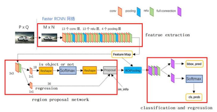
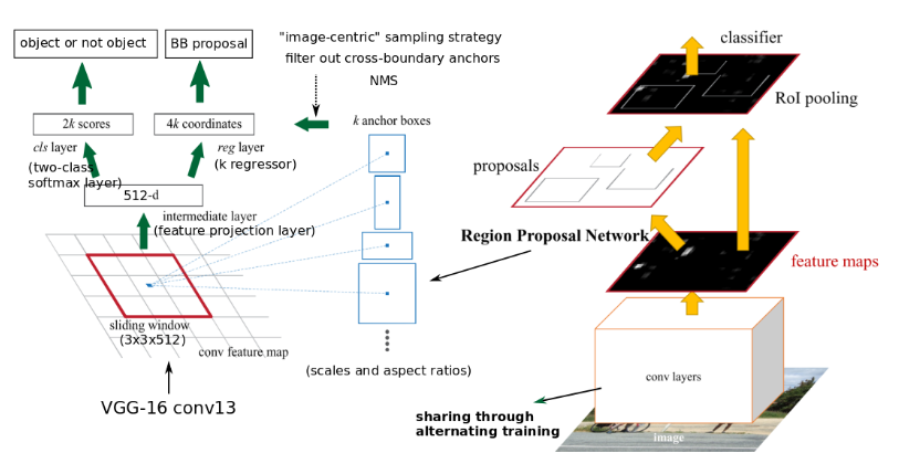
First, after the feature extraction operation is completed on the image, the result of FPN is obtained, that is, the Feature Map in the above figure is obtained after the final output of FPN through 3x3 convolution fusion. Then, operate on the result Feature Map of FPN: like the RPN in fast r-cnn, first perform 3 on × 3, and then on this result, two parallel 1 × 1 convolution kernel convolutes the classification (front background) and frame position information (xywh) respectively.
Then we take out the RPN results and classify them after RoIpooling.
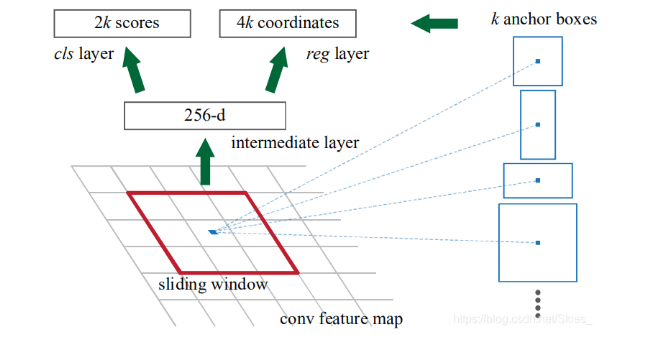
RPN is a series of sliding windows for target detection. Specifically, RPN is performed for 3 years first × 3, followed by two parallel ones × 1 convolution, distribution produces background classification and frame position regression. We call this combination network head.
FPN for RPN
RPN is a series of sliding windows for target detection. Specifically, RPN is performed for 3 years first × 3, followed by two parallel ones × 1 convolution, distribution produces background classification and frame position regression. We call this combination network head.
However, the front background classification and box position regression are carried out on the basis of anchor. In short, we first define some boxes, and then RPN can adjust them based on these boxes. In SSD, anchor is called prior, which is more vivid. In order to make regression easier, anchor predicted three sizes of scale s and three ratios of width to height in fast r-cnn, ratio{1:1, 1:2, 2:1}, with a total of 3 * 3 = 9 anchor frames.
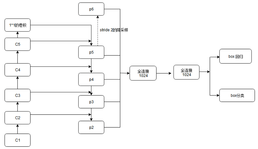
We also use a 3 in FPN × 3 and two parallel 1 × 1. However, RPN is performed on each level. Since FPN already has feature scales of different sizes, we don't need to use anchors of three sizes like fast r-cnn. Therefore, fix the anchor size corresponding to the feature map of each layer, and then use boxes of three ratios. In other words, the author applies a single-scale anchor at each pyramid level. The corresponding anchor scales of {P2, P3, P4, P5 and P6} are {32 * 32, 64 * 64, 128 * 128, 256 * 256 and 512 * 512}. Of course, the targets cannot all be square, so three comparative examples are still used ` ` {1:2, 1:1 and 2:1} ` ` ` ` `, so there are 15 kinds of anchors in the pyramid structure.
Selection of positive and negative samples in RPN network
RPN network needs to have the label that anchor is the foreground or background during training. Therefore, it is necessary to classify anchor into positive and negative samples. The principle is the same as that in fast r-cnn.
The specific methods are as follows: IoU > 0.7 of anchor and gt is a positive sample (label=1), IoU < 0.3 is a negative sample (label=0), and the rest between 0.3 and 0.7 are directly discarded and do not participate in training (label=-1). For example, after training 256 anchors in fast r-cnn, we get W × H × 9 roi.
In addition, the parameters of the header of each level are shared, and the reason for sharing is verified by experiments. Experiments show that although the feature size of each level is different, the accuracy of sharing and not sharing header parameters is similar. This result also shows that in fact, each level of the pyramid has almost similar semantic information, rather than the semantic information of ordinary networks.
FPN for Fast R-CNN
After the RPN network extracts the features, Fast R-CNN extracts the ROI with RoIpool and classifies it. RoIpool in Fast R-CNN is used to extract the features. Fast R-CNN performs well on single scale features. In order to use FPN, you need to assign the ROI of each scale to the pyramid level. The ROI pooling layer in Fast R-CNN uses the results and characteristic map of RPN as input. Through the feature pyramid, we get many feature maps. The author believes that the size of objects contained in different levels of feature maps is also different. Therefore, for ROI of different scales, different feature layers are used as the input of ROI pooling layer. Large scale ROI uses the later pyramid layers, such as P5; Small scale ROI uses the feature layer of the previous point, such as P4.
For W on the original drawing × For the RoI of H, you need to select the feature map of one layer to pool him. The number of layers of the selected feature map is P_k is selected based on:
224 is the size of ImageNet pre training, K0 is the reference value, set to 5 or 4, representing the output of P5 layer (P5 layer is used for the size of the original image), W and H are the length and width of ROI area. Assuming that ROI is 112 * 112, k = k0-1 = 5-1 = 4, which means that the ROI should use P4 feature layer. K value is rounded. This means that if the scale of ROI becomes smaller (such as 1 / 2 of 224), it should be mapped to a fine resolution level.
import torch
import torch.nn.functional as F
import torch.nn as nn

class FPN(nn.Module):
    def __init__(self,in_channel_list,out_channel):
        super(FPN, self).__init__()
        self.inner_layer=[]
        self.out_layer=[]
        for in_channel in in_channel_list:
            self.inner_layer.append(nn.Conv2d(in_channel,out_channel,1))
            self.out_layer.append(nn.Conv2d(out_channel,out_channel,kernel_size=3,padding=1))
        # self.upsample=nn.Upsample(size=, mode='nearest')
    def forward(self,x):
        head_output=[]
        corent_inner=self.inner_layer[-1](x[-1])
        head_output.append(self.out_layer[-1](corent_inner))
        for i in range(len(x)-2,-1,-1):
            pre_inner=corent_inner
            corent_inner=self.inner_layer[i](x[i])
            size=corent_inner.shape[2:]
            pre_top_down=F.interpolate(pre_inner,size=size)
            add_pre2corent=pre_top_down+corent_inner
            head_output.append(self.out_layer[i](add_pre2corent))
        return list(reversed(head_output))

if __name__ == '__main__':
    fpn=FPN([10,20,30],5)
    x=[]
    x.append(torch.rand(1, 10, 64, 64))
    x.append(torch.rand(1, 20, 16, 16))
    x.append(torch.rand(1, 30, 8, 8))
    c=fpn(x)
    print(c)
RPN architecture and its pytoch implementation
The following figure shows the RPN structure given by fast r-cnn:
Generate ~ 20k candidate frames based on RPN
Let's start with H × W × 9 Anchor codes.
Firstly, nine anchors are generated for the top left corner of the feature graph.
# anchor is generated for the top left corner of the feature graph
def generate_base_anchor(base_size=16, ratios=None, anchor_scale=None):
    """
    It is assumed that the size of the obtained characteristic graph is w×h,A total of 9 are generated at each location anchor,So there are anchor
    Number is w×h×9. In the original paper anchor The ratio is 1:2,2:1 And 1:1,Scales 128, 256, and 512 (relative to
    In terms of the original drawing). Therefore, the actual scales on the feature map sampled at 16 times are 8, 16 and 32.
    """
    # Ratio and scale of anchor
    if anchor_scale is None:
        anchor_scale = [8, 16, 32]
    if ratios is None:
        ratios = [0.5, 1, 2]
    # The position of the upper left corner of the feature map is mapped back to the position of the original map
    py = base_size / 2
    px = base_size / 2
    # Initialization variable (9,4). Here, take the top left corner vertex of the feature graph as an example to generate anchor
    base_anchor = np.zeros((len(ratios) * len(anchor_scale), 4), dtype=np.float32)
    # The loop generates 9 anchor s
    for i in range(len(ratios)):
        for j in range(len(anchor_scale)):
            # Generate height and width (relative to the original)
            # Take i=0, j=0 as an example, h=16 × eight × (0.5)^1/2,w=16 × eight × 1 / 0.5, then h × w=128^2
            h = base_size * anchor_scale[j] * np.sqrt(ratios[i])
            w = base_size * anchor_scale[j] * np.sqrt(1. / ratios[i])
            # Index of currently generated anchor (0 ~ 8)
            index = i * len(anchor_scale) + j
            # Calculate the upper left and lower right coordinates of anchor
            base_anchor[index, 0] = py - h / 2
            base_anchor[index, 1] = px - w / 2
            base_anchor[index, 2] = py + h / 2
            base_anchor[index, 3] = px + w / 2
    # Anchor relative to the original size (x_min, y_min, x_max, y_max)
    return base_anchor
Call the above function to see the printed results:
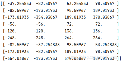
Take the first behavior example of the result graph to illustrate (don't care about those anchors that cross the boundary for now). First calculate its width and height:
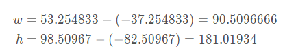
Then calculate its area:
From the width, height and area of the Anchor, we can see that it is an Anchor with a size of 128 and a ratio of 1:2. The above function is the Anchor generated by mapping the top left corner of the feature graph back to the original graph. We need the result of the whole feature graph. The following functions are defined:
def generate_all_base_anchor(base_anchor, feat_stride, height, width):
    """
    height*feat_stride/width*feat_stride Equivalent to the height of the original drawing/Width, equivalent to starting from 0,
    every other feat_stride=16 Sampling a position, which is equivalent to gradually sampling on the feature map sampled at 16 times. this
    A process is used to identify each group anchor The center point of the.
    """
    # Longitudinal offset [0,16,32,...]
    shift_y = np.arange(0, height * feat_stride, feat_stride)
    # Lateral offset [0,16,32,...]
    shift_x = np.arange(0, width * feat_stride, feat_stride)
    # np.meshgrid is used to change two one-dimensional vectors into two two-dimensional matrices. Where, the first 2D returned
    # The row vector of the matrix is the first parameter and the number of repetitions is the length of the second parameter; Column vector of the second two-dimensional matrix
    # Is the second parameter and the number of repetitions is the length of the first parameter. The resulting shift_x and shift_y as follows:
    # shift_x = [[0,16,32,...],
    #            [0,16,32,...],
    #            [0,16,32,...],
    #            ...]
    # shift_y = [[0, 0, 0,... ],
    #            [16,16,16,...],
    #            [32,32,32,...],
    #            ...]
    # Notice the shift_x and shift_y is equal to the scale of the feature graph, and the of each position corresponds to the scale of the feature graph
    # The combination of the values of the two matrices corresponds to the point on the characteristic graph mapped back to the upper left corner coordinate of the original graph.
    shift_x, shift_y = np.meshgrid(shift_x, shift_y)
    # NP. Travel () expands the matrix into a one-dimensional vector, shift_x and shift_ The expanded forms of Y are:
    # [0,16,32,...,0,16,32,..,0,16,32,...],(1,w*h)
    # [0,0,0,...,16,16,16,...,32,32,32,...],(1,w*h)
    # axis=0 is equivalent to stacking by line, and the shape obtained is (4,w*h);
    # axis=1 is equivalent to stacking by column, and the resulting shape is (w*h,4). The value of shift obtained by this statement is:
    # [[0,  0, 0,  0],
    #  [16, 0, 16, 0],
    #  [32, 0, 32, 0],
    #  ...]
    shift = np.stack((shift_y.ravel(), shift_x.ravel(),
                      shift_y.ravel(), shift_x.ravel()), axis=1)

    # Number of anchor s per location
    num_anchor_per_loc = base_anchor.shape[0]
    # Gets the total number of positions on the feature graph
    num_loc = shift.shape[0]
    # Use generate_ base_ The anchor at the upper left corner generated by anchor can be obtained by adding the offset
    # The following anchor information (here only refers to the change of anchor center point position, not the change of anchor)
    # Width and height). We first define the shape of the final anchor. We know that it should be w*h*9, then all
    # The stored variables of anchor are (w*h*9,4). First, the anchor shape generated by the first position is changed to
    # (1, 9, 4), and then change the shape of the shift to (1,w*h,4). And change it through the transfer function
    # The shape of the shift is (w*h,1,4), and then the broadcast mechanism is used to add the two, that is, the shape of the two is divided
    # Do not be (1,num_anchor_per_loc,4)+(num_loc,1,4), and finally add the result
    # The shape is (num_loc,num_anchor_per_loc,4). Here, the first item added is:
    # [[[x_min_0,y_min_0,x_max_0,y_max_0],
    #   [x_min_1,y_min_1,x_max_1,y_max_1],
    #   ...,
    #   [x_min_8,y_min_8,x_max_8,y_max_8]]]
    # The second item added is:
    # [[[0,  0, 0,  0]],
    #  [[0, 16, 0, 16]],
    #  [[0, 32, 0, 32]],
    #  ...]
    # In the process of addition, we first expand the two addends into the target shape. Specifically, the first one can
    # Expand to:
    # [[[x_min_0,y_min_0,x_max_0,y_max_0],
    #   [x_min_1,y_min_1,x_max_1,y_max_1],
    #   ...,
    #   [x_min_8,y_min_8,x_max_8,y_max_8]],
    #  [[x_min_0,y_min_0,x_max_0,y_max_0],
    #   [x_min_1,y_min_1,x_max_1,y_max_1],
    #   ...,
    #   [x_min_8,y_min_8,x_max_8,y_max_8]],
    #  [[x_min_0,y_min_0,x_max_0,y_max_0],
    #   [x_min_1,y_min_1,x_max_1,y_max_1],
    #   ...,
    #   [x_min_8,y_min_8,x_max_8,y_max_8]],
    #   ...]
    # The second can be expanded to:
    # [[[0,  0, 0,  0],
    #   [0,  0, 0,  0],
    #   ...],
    #  [[0, 16, 0, 16],
    #   [0, 16, 0, 16],
    #   ...],
    #  [[0, 32, 0, 32],
    #  [0, 32, 0, 32],
    #  ...],
    #  ...]
    # Now the two dimensions are consistent and can be added directly. The resulting shape is:
    # (num_loc,num_anchor_per_loc,4)
    anchor = base_anchor.reshape((1, num_anchor_per_loc, 4)) + \
             shift.reshape((1, num_loc, 4)).transpose((1, 0, 2))
    # reshape the anchor shape to the final shape (num_loc*num_anchor_per_loc,4).
    anchor = anchor.reshape((num_loc * num_anchor_per_loc, 4)).astype(np.float32)
    return anchor
The above code has very detailed comments. Let's look at some of the more important functions.
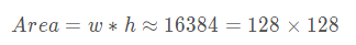
NP. Range (start = 0, end, step = 1): generate an equal difference array within the range of [start, end) in steps, such as:
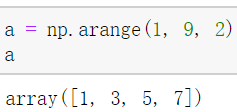
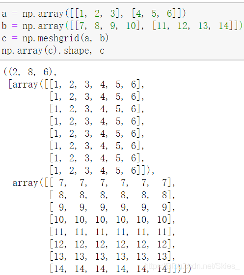
np.meshgrid(x, y): returns a (2, y.length(), x.length()) matrix based on vector x and vector y. here, if the parameter is not a one-dimensional vector, the function will first expand it into a one-dimensional vector by row. In addition, the expansion methods of elements are different: the first parameter is expanded by row and the second parameter is expanded by column. For example:
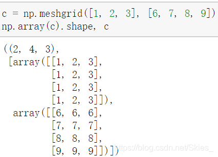
np.stack(arrays, axis=0): stack arrays in the dimension of axis=0. Let's first take one-dimensional vector as an example:
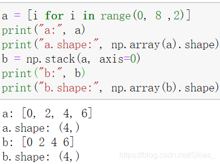
Since a has only one dimension, it will not change when using the stack function on itself. Now make the following changes:
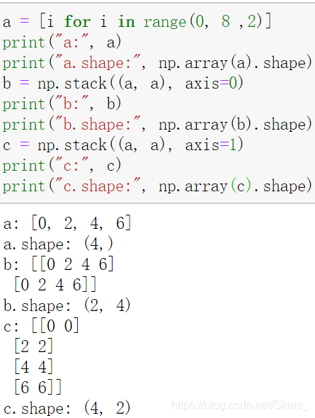
We can see that when axis=0, it is equivalent to stacking a by row; when axis=1, it is equivalent to stacking a by column. The same is true for other high-dimensional vectors.
Transfer(): transpose the matrix according to a certain law. The transposing method depends on the specific parameters. For example:
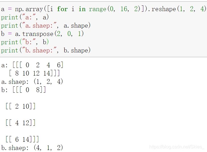
We first fix the shape of a as (1, 2, 4), and then call the function transfer to get b. because the original a.shape = (1, 2, 3) corresponds to the zeroth dimension, the first dimension and the second dimension, i.e. 0, 1, 2; transfer (2, 0, 1) It is equivalent to placing the element of the original zero dimension in the second position, the element of the first dimension in the third position, and the element of the second dimension in the first position, that is, it corresponds to shape: (1, 2, 4) = > (4, 1, 2). Other transformations are the same.
~20k candidate boxes (1): RPN
After about 20000 candidate frames are generated from the RPN, on the one hand, a part is selected for training the RPN. Specifically, 256 candidate frames are selected from about 20000 candidate frames, that is, 128 positive samples and 128 negative samples.
The selection process is as follows:
- For each real box, select the candidate box with the largest intersection union ratio as the positive sample. Obviously, because there are too few annotation targets in the figure, we can't meet the training requirements, so let's go through the following steps;
- For the remaining candidate frames, if the intersection union ratio with a real frame is greater than the set threshold, we also consider it a positive sample;
- At the same time, set a negative sample threshold. If the combat ratio between the candidate frame and the real frame is less than the threshold, it will be regarded as a negative sample.
- note that when selecting positive samples and negative samples, the quantity requirements shall be strictly met.
class AnchorTargetCreator(object):
    def __init__(self, n_sample=256, pos_iou_thresh=0.7, neg_iou_thresh=0.3, pos_ratio=0.5):
        # Total samples
        self.n_sample = n_sample
        # Threshold of positive and negative samples
        self.pos_iou_thresh = pos_iou_thresh
        self.neg_iou_thresh = neg_iou_thresh
        # Positive and negative sample sampling ratio
        self.pos_ratio = pos_ratio

    def __call__(self, bbox, anchor, img_size):
        img_H, img_W = img_size
        # ~20k anchor s
        n_anchor = len(anchor)
        # Only legal anchors are retained
        inside_index = _get_inside_index(anchor, img_H, img_W)
        anchor = anchor[inside_index]
        # Returns the maximum intersection union ratio index corresponding to each anchor and bbox and the positive and negative sample sampling results
        argmax_ious, label = self._create_label(inside_index, anchor, bbox)
        # Calculate regression target
        loc = bbox2loc(anchor, bbox[argmax_ious])
        # The candidate box is obtained according to the index
        label = _unmap(label, n_anchor, inside_index, fill=-1)
        loc = _unmap(loc, n_anchor, inside_index, fill=0)
        return loc, label

    def _create_label(self, inside_index, anchor, bbox):
        # label: 1 indicates positive sample index, 0 indicates negative sample, and - 1 indicates ignore
        label = np.empty((len(inside_index),), dtype=np.int32)
        label.fill(-1)
        # Returns the maximum intersection union ratio and index corresponding to each anchor and bbox, as well as the positive sample index generated in the first step
        argmax_ious, max_ious, gt_argmax_ious = self._calc_ious(anchor, bbox, inside_index)
        # If the maximum intersection union ratio is less than the threshold, the negative sample is selected first
        label[max_ious < self.neg_iou_thresh] = 0
        # Positive sample generated in the first step
        label[gt_argmax_ious] = 1
        # Positive samples generated in the second step
        label[max_ious >= self.pos_iou_thresh] = 1
        # If the number of positive samples is greater than 128, random sampling again
        n_pos = int(self.pos_ratio * self.n_sample)
        pos_index = np.where(label == 1)[0]
        if len(pos_index) > n_pos:
            disable_index = np.random.choice(
                pos_index, size=(len(pos_index) - n_pos), replace=False)
            label[disable_index] = -1
        # If the number of negative samples is greater than 128, random sampling again
        n_neg = self.n_sample - np.sum(label == 1)
        neg_index = np.where(label == 0)[0]
        if len(neg_index) > n_neg:
            disable_index = np.random.choice(
                neg_index, size=(len(neg_index) - n_neg), replace=False)
            label[disable_index] = -1
        return argmax_ious, label

    def _calc_ious(self, anchor, bbox, inside_index):
        # Calculate the intersection and union ratio between anchor and bbox, and return the shape as (len(anchor),len(bbox))
        # That is, a two-dimensional matrix reflects the intersection and union ratio between anchor and bbox
        ious = bbox_iou(anchor, bbox)
        # For each anchor, find the index of the bbox with the largest intersection union ratio
        # axis=1 find the maximum value by column, and the returned shape is (1,len(bbox))
        argmax_ious = ious.argmax(axis=1)
        max_ious = ious[np.arange(len(inside_index)), argmax_ious]
        # For each bbox, find the index of the anchor with the largest intersection union ratio
        # axis=0, find the maximum value by line, and the returned shape is (len(anchor),1)
        gt_argmax_ious = ious.argmax(axis=0)
        gt_max_ious = ious[gt_argmax_ious, np.arange(ious.shape[1])]
        # Corresponding to the first step of selecting positive samples, the anchor with the largest intersection union ratio with bbox is the positive sample, and its index is obtained
        gt_argmax_ious = np.where(ious == gt_max_ious)[0]
        return argmax_ious, max_ious, gt_argmax_ious
Among them, bbox2loc is a function to calculate the offset according to the real box and the candidate box. The formula is as follows:

def bbox2loc(src_bbox, dst_bbox):
    # Prediction frame (xmin, Ymin, xmax, ymax) = > (x, y, W, H)
    height = src_bbox[:, 2] - src_bbox[:, 0]
    width = src_bbox[:, 3] - src_bbox[:, 1]
    ctr_y = src_bbox[:, 0] + 0.5 * height
    ctr_x = src_bbox[:, 1] + 0.5 * width
    # Real box (xmin, Ymin, xmax, ymax) = > (x, y, W, H)
    base_height = dst_bbox[:, 2] - dst_bbox[:, 0]
    base_width = dst_bbox[:, 3] - dst_bbox[:, 1]
    base_ctr_y = dst_bbox[:, 0] + 0.5 * base_height
    base_ctr_x = dst_bbox[:, 1] + 0.5 * base_width
    # Minimum value to ensure that the divisor is not zero
    eps = np.finfo(height.dtype).eps
    height = np.maximum(height, eps)
    width = np.maximum(width, eps)
    # apply a formula
    dy = (base_ctr_y - ctr_y) / height
    dx = (base_ctr_x - ctr_x) / width
    dh = np.log(base_height / height)
    dw = np.log(base_width / width)
    # Stack results
    loc = np.vstack((dy, dx, dh, dw)).transpose()
    return loc
~20k candidate boxes (2): Fast R-CNN
After about 20000 candidate frames are generated by RPN, on the other hand, some are selected for training fast RCNN. Here, the number of candidate frames selected and processed in the training stage and reasoning stage is different. In the training stage, about 12k candidate frames are selected and about 2k candidate frames are obtained by non maximum suppression; In the reasoning stage, about 6k candidate frames are selected, and about 0.3k candidate frames are obtained by non maximum suppression. The rule selected here is the classification confidence of the candidate box.
class ProposalCreator:
    def __init__(self, parent_model, nms_thresh=0.7, n_train_pre_nms=12000, n_train_post_nms=2000,
                 n_test_pre_nms=6000, n_test_post_nms=300, min_size=16):
        self.parent_model = parent_model
        self.nms_thresh = nms_thresh
        self.n_train_pre_nms = n_train_pre_nms
        self.n_train_post_nms = n_train_post_nms
        self.n_test_pre_nms = n_test_pre_nms
        self.n_test_post_nms = n_test_post_nms
        self.min_size = min_size

    def __call__(self, loc, score, anchor, img_size, scale=1.):
        # Different numbers of candidate boxes are used in the training phase and reasoning phase
        if self.parent_model.training:
            n_pre_nms = self.n_train_pre_nms
            n_post_nms = self.n_train_post_nms
        else:
            n_pre_nms = self.n_test_pre_nms
            n_post_nms = self.n_test_post_nms
        # The actual information of anchor is obtained according to the offset
        roi = loc2bbox(anchor, loc)
        # Limit the width and height of the prediction box to the preset range
        roi[:, slice(0, 4, 2)] = np.clip(
            roi[:, slice(0, 4, 2)], 0, img_size[0])
        roi[:, slice(1, 4, 2)] = np.clip(
            roi[:, slice(1, 4, 2)], 0, img_size[1])
        min_size = self.min_size * scale
        hs = roi[:, 2] - roi[:, 0]
        ws = roi[:, 3] - roi[:, 1]
        keep = np.where((hs >= min_size) & (ws >= min_size))[0]
        roi = roi[keep, :]
        score = score[keep]
        # Sort to get the candidate box of the high confidence part
        order = score.ravel().argsort()[::-1]
        if n_pre_nms > 0:
            order = order[:n_pre_nms]
        roi = roi[order, :]
        score = score[order]
        # The nms process is not expanded in detail here. pytorch1.2 + can be directly used by importing nms through from torchvision.ops import
        keep = nms(torch.from_numpy(roi).cuda(), torch.from_numpy(score).cuda(), self.nms_thresh)
        if n_post_nms > 0:
            keep = keep[:n_post_nms]
        roi = roi[keep.cpu().numpy()]
        # Returns the generated candidate box
        return roi
After the candidate box is finally selected through non maximum suppression, the following work is the content of fast RCNN, which will not be introduced here. Among them, the loc2bbox function is the inverse process of the bbox2loc function, that is, the real box value is obtained according to the offset.
RPN body
RPN has outputs in two directions. On the one hand, two branches are obtained by convolution in the RPN part, namely classification and regression; On the other hand, candidate regions are generated as input to the fast RCNN part. The following is the specific code:
class RegionProposalNetwork(nn.Module):
    def __init__(self, in_channels=512, mid_channels=512, ratios=[0.5, 1, 2],
                 anchor_scales=[8, 16, 32], feat_stride=16,
                 proposal_creator_params=dict(), ):
        super(RegionProposalNetwork, self).__init__()
        # anchor corresponding to the top left corner of the feature graph
        self.anchor_base = generate_anchor_base(anchor_scales=anchor_scales, ratios=ratios)
        # Down sampling multiple
        self.feat_stride = feat_stride
        # Generate candidate boxes for Fast RCNN
        self.proposal_layer = ProposalCreator(self, **proposal_creator_params)
        n_anchor = self.anchor_base.shape[0]
        self.conv1 = nn.Conv2d(in_channels, mid_channels, 3, 1, 1)
        self.score = nn.Conv2d(mid_channels, n_anchor * 2, 1, 1, 0)
        self.loc = nn.Conv2d(mid_channels, n_anchor * 4, 1, 1, 0)
        # Weight initialization
        normal_init(self.conv1, 0, 0.01)
        normal_init(self.score, 0, 0.01)
        normal_init(self.loc, 0, 0.01)

    def forward(self, x, img_size, scale=1.):
        n, _, hh, ww = x.shape
        # Generate all anchor s
        anchor = _enumerate_shifted_anchor(np.array(self.anchor_base), self.feat_stride, hh, ww)
        n_anchor = anchor.shape[0] // (hh * ww)
        # Regression branch of rpn part
        h = F.relu(self.conv1(x))
        rpn_locs = self.loc(h)
        rpn_locs = rpn_locs.permute(0, 2, 3, 1).contiguous().view(n, -1, 4)
        # Classification branch of rpn part
        rpn_scores = self.score(h)
        rpn_scores = rpn_scores.permute(0, 2, 3, 1).contiguous()
        rpn_softmax_scores = F.softmax(rpn_scores.view(n, hh, ww, n_anchor, 2), dim=4)
        rpn_fg_scores = rpn_softmax_scores[:, :, :, :, 1].contiguous()
        rpn_fg_scores = rpn_fg_scores.view(n, -1)
        rpn_scores = rpn_scores.view(n, -1, 2)
        # Generate rois part
        rois = list()
        roi_indices = list()
        for i in range(n):
            roi = self.proposal_layer(
                rpn_locs[i].cpu().data.numpy(),
                rpn_fg_scores[i].cpu().data.numpy(),
                anchor, img_size,
                scale=scale)
            batch_index = i * np.ones((len(roi),), dtype=np.int32)
            rois.append(roi)
            roi_indices.append(batch_index)
        rois = np.concatenate(rois, axis=0)
        roi_indices = np.concatenate(roi_indices, axis=0)
        return rpn_locs, rpn_scores, rois, roi_indices, anchor
Loss function of RPN part
The overall loss function of fast r-cnn is defined as follows:

Among them, the first part is classified loss, N_{cls} represents the total number of samples calculated by the classification branch. Here, the values of RPN and Fast R-CNN are different; The second part is regression loss, N_{cls} represents the total number of samples calculated by the regression branch. Where, the regression loss is multiplied by a p_i ^ * indicates that the regression loss is only for positive samples. The cross entropy loss is used in the classification loss part, and the SmoothL1 loss is used in the regression loss part.
First, let's look at the part of manually realizing SmoothL1 loss:
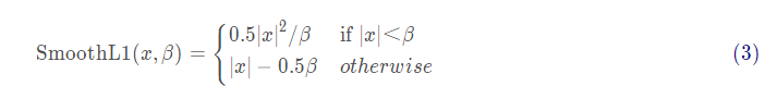
def _smooth_l1_loss(x, t, in_weight, sigma):
    # Equivalent to 1 in the formula/ β
    sigma2 = sigma ** 2
    # It is equivalent to | x in the formula|
    diff = in_weight * (x - t)
    abs_diff = diff.abs()
    # Equivalent to the judgment conditions in the formula
    flag = (abs_diff.data < (1. / sigma2)).float()
    # Select different branches for calculation according to the range of | x |
    y = (flag * (sigma2 / 2.) * (diff ** 2) +
         (1 - flag) * (abs_diff - 0.5 / sigma2))
    return y.sum()

def _fast_rcnn_loc_loss(pred_loc, gt_loc, gt_label, sigma):
    in_weight = torch.zeros(gt_loc.shape).cuda()
    in_weight[(gt_label > 0).view(-1, 1).expand_as(in_weight).cuda()] = 1
    loc_loss = _smooth_l1_loss(pred_loc, gt_loc, in_weight.detach(), sigma)
    # The loss value is normalized by the total number of samples involved in the calculation
    loc_loss /= ((gt_label >= 0).sum().float())
    return loc_loss
Then is the main part of calculating the loss function of the RPN part:
class FasterRCNNTrainer(nn.Module):
    def __init__(self, faster_rcnn):
        super(FasterRCNNTrainer, self).__init__()
        self.faster_rcnn = faster_rcnn
        # Parameters of smoothl1 loss function
        self.rpn_sigma = 3
        # The samples of rpn part participating in loss calculation are obtained
        self.anchor_target_creator = AnchorTargetCreator()

    def forward(self, imgs, bboxes, labels, scale):
        # Only batch is supported_ Calculation of size = 1
        n = bboxes.shape[0]
        if n != 1:
            raise ValueError('Currently only batch size 1 is supported.')
        _, _, H, W = imgs.shape
        img_size = (H, W)
        # Feature map generated by cnn
        features = self.faster_rcnn.extractor(imgs)
        # Candidate frame generated by rpn
        rpn_locs, rpn_scores, rois, roi_indices, anchor = \
            self.faster_rcnn.rpn(features, img_size, scale)
        # Since batch size is one, convert variables to singular form
        bbox = bboxes[0]
        rpn_score = rpn_scores[0]
        rpn_loc = rpn_locs[0]
        # rpn_loss
        gt_rpn_loc, gt_rpn_label = self.anchor_target_creator(
            at.tonumpy(bbox), anchor, img_size)
        gt_rpn_label = at.totensor(gt_rpn_label).long()
        gt_rpn_loc = at.totensor(gt_rpn_loc)
        # Regression loss, call the custom smoothl1 loss function
        rpn_loc_loss = _fast_rcnn_loc_loss(
            rpn_loc, gt_rpn_loc, gt_rpn_label.data, self.rpn_sigma)
        # Classification loss, call the cross entropy loss function of pytorch
        rpn_cls_loss = F.cross_entropy(rpn_score, gt_rpn_label.cuda(), ignore_index=-1)
        _gt_rpn_label = gt_rpn_label[gt_rpn_label > -1]
        _rpn_score = at.tonumpy(rpn_score)[at.tonumpy(gt_rpn_label) > -1]
        return rpn_loc_loss, rpn_cls_loss