catalogue
1. Introduction to discrete Laplace operator
3. Introduction to solution of Possion equation
IV. algorithm implementation in Python
1. Define the function calMSE calculation error Mean Square Error
2. Import the original drawing and note the size
4. Convolution and DCT transform
6. Inverse transform, pull back the low frequency and display.
7. Printing error and time consuming
1, Background
The digitized image data occupies a very large space. We might as well calculate the following: a 32-bit gray image with a resolution of 800 * 600 pixels, the number of pixels is 480000, and the occupied space is 480000*32bit=480000*4B ≈ 1.83MB. Assuming a movie frame rate of 24 frames per second, it takes 1.83*24=43.92MB to store a movie for one second at this resolution. At present, most use cases are color pictures in three channels. Then multiply this number by 3 and it is only one second. You can imagine how huge the amount of data is.
The size of image data creates great difficulties for image storage and transmission. Image compression is to remove the redundant information of the image and realize effective compression. For example, the feature map can retain the relative situation of each position, and the discrete Fourier transform can concentrate the data in low frequency and so on. In this paper, only the characteristic image is used to compress the "image" data, and the solution of Poisson equation is used to reconstruct the image
2, Principle
1. Introduction to discrete Laplace operator
The derivative of the discrete function degenerates into difference. The one-dimensional first-order difference formula and second-order formula are respectively:

The Laplace operator of the discrete function is obtained by the difference of the second derivative of the Laplace operator in X and Y directions
In a two-dimensional function f (x, y), the second-order differences in the two directions of X and y are:

Therefore, the difference form of Laplace operator is:

In the form of convolution kernel:
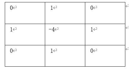
Of course, it can also be written as follows:
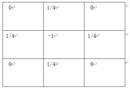
Note the characteristics of the core. The results of the mask are the same in the four 90 ° directions, that is, there is no directivity in the 90 ° direction. In order to make the mask have this property at 45 °, we introduce another convolution kernel:
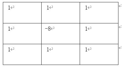
These are the two most common Laplace convolution kernels. Another common convolution kernel will be introduced below:
The operation of the so-called convolution kernel is nothing more than moving line by line on the original image like spatial filtering, multiplying the value on the kernel by its coincident pixels, summing, and finally assigning the calculated value to the copy position corresponding to the core center. For the first and last rows / columns of the image, we cannot calculate them uniformly. Here, we introduce two solutions:
- Laplace graph is two rows and two columns smaller than the original graph or stores 0
- Expanding the original graph into a graph of M+2 and N+2 is equal to adding a border of one pixel to the original graph. This box is assigned 0 or the nearest row / column
Corresponding to the two methods in 2, that is, the conditions of the first type of boundary conditions (Dirichlet boundary) and the second type of Newman boundary are artificially given. At this time, there are two solutions. In solution 1, although the size problem of the graph is solved, no boundary conditions are given, so it can not be solved numerically by discrete cosine / sine transform, but it can be solved by solving the coefficient matrix. In this experiment, discrete Fourier transform is used, so the second scheme is adopted
2. Laplace convolution
Back to the point, now give a 4 * 4 size diagram:
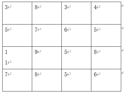
According to the first convolution introduced above: (the original drawing is OriginalPic, abbreviated as O below)
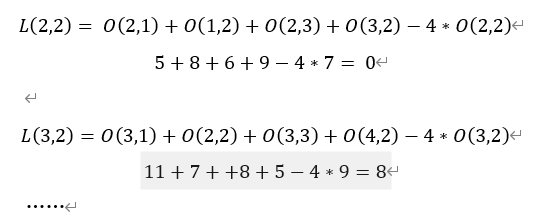
We can get the following Laplace diagram
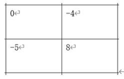
In this way, four equations can be listed:

What we require is the pixel values of each point in the original image, but it is impossible to solve 16 unknowns in four equations, so we add constraints. For example, if we know the values of 12 boundaries (Dirichlet boundary condition), we can get another 12 equations. In this way, when 16 equations solve 16 unknowns, we can easily solve them in python. However, we want to use the dct and dst transformations described below:
Taking dct as an example, assuming that we already know the Newman boundary condition, that is, the gradient of the boundary, we need to expand the above 4 * 4 to 6 * 6, as follows:
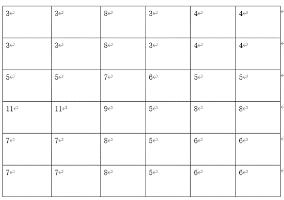
In this way, the characteristic diagram we obtained is:
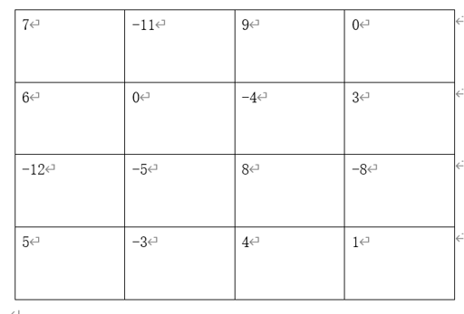
3. Introduction to solution of Possion equation
null https://elonen.iki.fi/code/misc-notes/neumann-cosine/index.html From ↑ ↑ ↑
How to reconstruct the original image from feature map? This requires the Poisson equation solution:
The 2D Poisson equation in the continuous domain is in the following form:

The discrete domain form is:( μ Original drawing, ρ Characteristic diagram (LaplacePic mentioned above)

The function u (x, y) can be expressed as:

So we can get:

Our goal is to solve u. Two abbreviations are introduced to facilitate calculation:
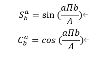
List the calculation formulas of 2D DST and its inverse 2D IDST Transformation:
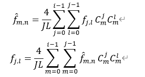
Substitute into both sides of the finite difference equation and eliminate the summation symbol to obtain the frequency domain equation:

Again

So:
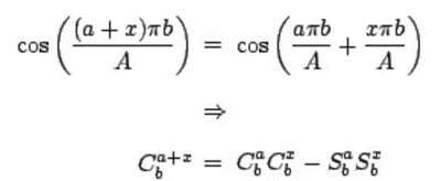
Again
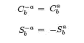
In order to solve μ^, Simplified equation form:


Therefore:

By substituting the original abbreviation, you can get:

According to the above derivation, solving Poisson equation is generally divided into four steps:
- The original image is convoluted to form a characteristic image according to the above method ρ
- yes ρ Get 2D DCT ρ^
- yes ρ^ Each pixel divided by the denominator 2 (COS( Π m/J)+cos( Π n/L)-2)
- Finally, through the ρ^ 2D IDCT transform reconstruction μ (original)
III. verification
Well, the principle is clear. Let's manually verify that the accuracy is 0.1. DCT transformation is performed on the above characteristic diagram to obtain:
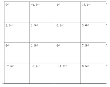
Divide by the denominator to get:
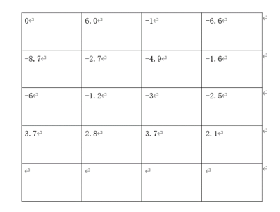
2D IDCT transform:
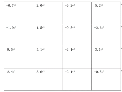
Finally, don't forget to subtract the average value of this figure and add the average value of the original figure. The purpose of this step is that this scheme can only restore the relative quantity, not the low-frequency component, so there must be the operation of pulling back the level line in the last step. The average value in this drawing is 0.65, and the average value in the original drawing is 6.25. After drawing and shaping, it is:
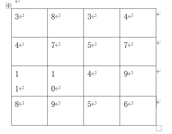
From the above results, it can be seen that although it is different from the original drawing, it is generally similar, which does not mean that the solution method is not good, the amount of data is small, and manual calculation errors are all error factors. On the graph with base number of 255, the gap is not large. The code implementation verification is carried out below.
IV. algorithm implementation in Python
a. DCT solution
1. Define the function calMSE calculation error Mean Square Error

2. Import the original drawing and note the size

3. Extended Original

4. Convolution and DCT transform

5. Divide by denominator

6. Inverse transform, pull back the low frequency and display.
There is a detail problem here. It is necessary to assign the value greater than 255 to 255 and the value less than 0 to 0 in the output diagram after being pulled up, otherwise the phenomenon of "black pole generates white and white pole generates black" will appear
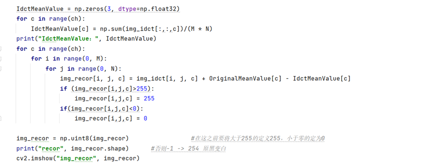
7. Printing error and time consuming

b. DST solution
In this way, the code implementation part is stated, but the above is the DCT solution method. For DST solution, due to the high similarity, only a brief discussion is made. Just change step 3 to:

The expanded boundary is assigned 0 and solved by Dirichlet boundary conditions. Then change step 5 to:

That is, the discrete sine under this condition is solved. Finally, the two forward and inverse transforms used in DCT can be changed into DST forward and inverse transform. But I didn't find the dst() function from cv2, so we used FFT in the scipy library DSTN () and FFT Replace with the idstn() function.
Although the solution methods under the above two boundary conditions can restore the feature image, the restoration accuracy is very different. The experimental verification shows that the processing speed of the two reconstruction methods is basically the same under different images.
So far, the whole experimental step is over
5, Error and result
Under DCT:
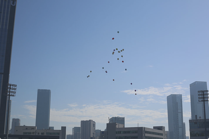
Original drawing:

Characteristic diagram:
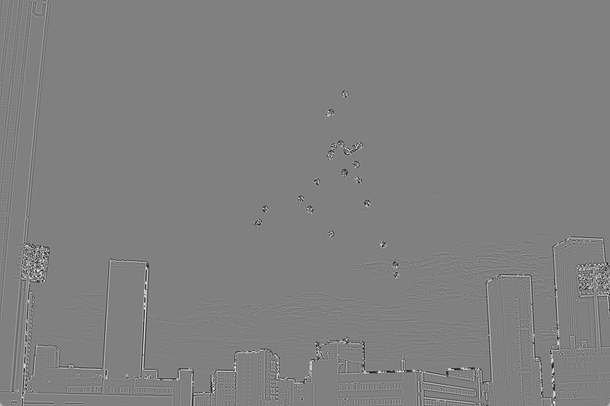
The first convolution kernel: (the three values of MSE correspond to the mean square deviation of the three channels respectively)

Time and error:

The mean square deviation is controlled within 0.4, and the image restoration is very successful.
Second: (the color is very dark and the reduction degree is not high)
Time and error:
Third:

Error and time consuming:

Vi. source code
import numpy as np
import cv2
import time
from scipy import fft

time_start = time.time()  # Start timing


# The function calMSE is defined to calculate the mean square error (MSE) evaluation index between the restoration map std and the target image aim
def calMSE(std, aim):
    # The mean square deviation of each channel is calculated cyclically
    num = np.zeros((std.shape[2]), dtype=np.float32)
    mse = np.zeros((std.shape[2]), dtype=np.float32)
    for c in range(std.shape[2]):
        for i in range(std.shape[0]):
            for j in range(std.shape[1]):
                num[c] += np.power(np.float32(std[i, j, c]) - np.float32(aim[i, j, c]), 2)  # A cast is required here
        mse[c] = np.sqrt(num[c] / (std.shape[0] * std.shape[1]))  # Otherwise, the error is small
    return mse


def main():
    img_cv = cv2.imread("D:/sy15.jpg")

    OriginalPic0 = np.array(img_cv, dtype=np.uint8)
    M, N, ch = OriginalPic0.shape  # M. N -- length and width (single channel)

    OriginalPic = np.zeros((OriginalPic0.shape[0] + 2, OriginalPic0.shape[1] + 2, 3), dtype=np.uint8)
    img_dct = np.zeros((M, N, ch), dtype=np.float32)
    img_idct = np.zeros((M, N, ch), dtype=np.float32)

    for c in range(ch):
        for i in range(1, M + 1):
            for j in range(1, N + 1):
                OriginalPic[i, j, c] = OriginalPic0[i - 1, j - 1, c]
        OriginalPic[:, 0, c] = OriginalPic[:, 1, c]
        OriginalPic[:, N + 1, c] = OriginalPic[:, N, c]
        OriginalPic[0, :, c] = OriginalPic[1, :, c]
        OriginalPic[M + 1, :, c] = OriginalPic[M, :, c]

    LaplacePic = np.zeros((M, N, ch), dtype=np.float32)  # Storage characteristic diagram
    LaplacePic_show = np.zeros((M, N, ch), dtype=np.uint8)  # Characteristic diagram to be displayed

    img_recor = np.zeros((M, N, ch), dtype=np.float32)

    OriginalMeanValue = np.zeros(3, dtype=np.float32)
    for c in range(ch):
        OriginalMeanValue[c] = np.sum(OriginalPic[:, :, c]) / (M * N)
    print("OriginalMeanValue: ", OriginalMeanValue)

    kernel1 = [[0, 1, 0], [1, -4, 1], [0, 1, 0]]  # Laplace convolution
    kernel2 = [[1 / 4, 1 / 4, 1 / 4], [1 / 4, -2, 1 / 4], [1 / 4, 1 / 4, 1 / 4]]  # Here, because the color difference is not obvious after reduction
    kernel3 = [[1 / 4, 1 / 2, 1 / 4], [1 / 2, -3, 1 / 2], [1 / 4, 1 / 2, 1 / 4]]  # Scale manually

    for c in range(ch):
        for i in range(1, M + 1):
            for j in range(1, N + 1):
                LaplacePic[i - 1][j - 1][c] = (np.sum(np.multiply(kernel3, OriginalPic[i - 1:i + 2, j - 1:j + 2, c])))
                LaplacePic_show[i - 1][j - 1][c] = LaplacePic[i - 1][j - 1][c] + 128  # Characteristic salience
        img_dct[:, :, c] = cv2.dct(LaplacePic[:, :, c])
    cv2.imshow("Original", OriginalPic)  # Show original
    cv2.imshow("Laplace", LaplacePic_show)  # Display feature map

    print("Original", OriginalPic0.shape)
    print("Laplace", LaplacePic.shape)

    for c in range(ch):
        for i in range(0, M):
            for j in range(0, N):
                img_dct[i, j, c] /= (2 * (np.cos(np.pi * i / (M + 2)) + np.cos(np.pi * j / (N + 2)) - 2))  # Divided by 2cos Π...
        img_dct[0, 0, c] = 0
        img_idct[:, :, c] = cv2.idct(img_dct[:, :, c])


    IdctMeanValue = np.zeros(3, dtype=np.float32)
    for c in range(ch):
        IdctMeanValue[c] = np.sum(img_idct[:, :, c]) / (M * N)
    print("IdctMeanValue: ", IdctMeanValue)
    for c in range(ch):
        for i in range(0, M):
            for j in range(0, N):
                img_recor[i, j, c] = img_idct[i, j, c] + OriginalMeanValue[c] - IdctMeanValue[c]
                if (img_recor[i, j, c] > 255):
                    img_recor[i, j, c] = 255
                if (img_recor[i, j, c] < 0):
                    img_recor[i, j, c] = 0

    img_recor = np.uint8(img_recor)  # Before that, define 255 greater than 255 and 0 less than zero
    print("recor", img_recor.shape)  # Otherwise - 1 - > 254 original black turns white
    cv2.imshow("img_recor", img_recor)

    MeanSquareError = calMSE(img_recor, OriginalPic0)
    print("MeanSquareError", MeanSquareError)

    time_end = time.time()  # End timing
    print("Time cost = %fs" % (time_end - time_start))
    cv2.waitKey(0)


if __name__ == '__main__':
    main()