preface
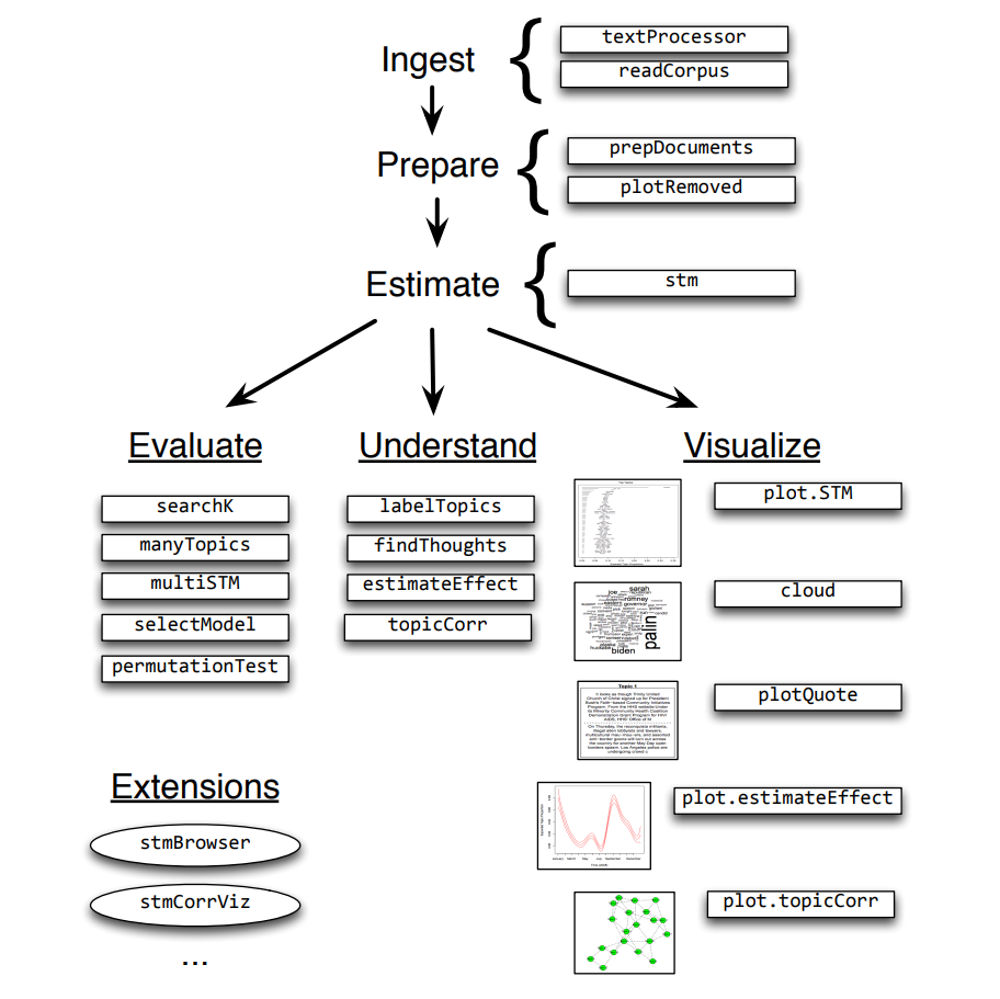
Sort out the workflow of STM code in the paper (stm: An R Package for Structural Topic Models). Refer to the original paper for the overall structure, but put forward personal ideas on the execution order of some codes. Due to the limited time, there are unsolved errors and problems (such as selecting the appropriate number of topics, drawing the time trend chart...), some contents at the back of the paper are not described in detail. I hope some friends can put forward effective suggestions for modification, and the blogger will give feedback at the first time. Finally, I hope it will be helpful to friends who use STM structure theme model 😁
3.0 reading data
Sample data: poliblogs2008 CSV is a collection of blog posts on American politics from CMU's 2008 political blog corpus: American Thinker, Digby, Hot Air, Michelle Malkin, Think Progress, and Talking Points Memo. Each blog forum has its own political tendency, so each blog has metadata of writing date and political ideology.
# data <- read.csv("./poliblogs2008.csv", sep =",", quote = "", header = TRUE, fileEncoding = "UTF-8")
data <- read_excel(path = "./poliblogs2008.xlsx", sheet = "Sheet1", col_names = TRUE)
Starting with 3.0, the serial number is to be consistent with the original paper
3.1 Ingest: Reading and processing text data
Extract data: process the original data into three pieces of content that STM can analyze (documents, vocab and meta respectively), using textProcessor or readCorpus.
The textProcessor() function is designed to provide a convenient and quick way to process relatively small text for analysis using software packages. It aims to quickly capture data in a simple form, such as a spreadsheet, where each document is located in a single cell.
# Call the textProcessor algorithm and take data$document and data as parameters
processed <- textProcessor(documents = data$documents, metadata = data)
It is mentioned in the paper that textProcessor() can handle multiple languages, and the variable language = "en" and customstopwords = null need to be set,. The blogger did not try
See: textProcessor function - RDocumentation
3.2 Prepare: Associating text with metadata
Data preprocessing: convert the data format, delete low-frequency words according to the threshold, and use two functions: prepDocuments() and plotRemoved()
The plotRemoved() function can plot the number of document s, words and token s deleted under different thresholds
pdf("output/stm-plot-removed.pdf")
plotRemoved(processed$documents, lower.thresh = seq(1, 200, by = 100))
dev.off()
According to the result of this pdf file (output/stm-plot-removed.pdf), determine the parameter lower. In prepDocuments() The value of thresh is used to determine the variables docs, vocab and meta
It is mentioned in the paper that if any changes occur during processing, PrepDocuments will also re index all metadata / document relationships. For example, when a document is completely deleted in the preprocessing phase because it contains low-frequency words, PrepDocuments() will also delete the corresponding lines in the metadata. Therefore, after reading and processing text data, it is important to check the characteristics of documents and related vocabulary to ensure that they have been preprocessed correctly.
# Remove words with word frequency less than 15
out <- prepDocuments(documents = processed$documents, vocab = processed$vocab, meta = processed$meta, lower.thresh = 15)

docs <- out$documents
vocab <- out$vocab
meta <- out$meta
-
docs: documents. A list of documents containing word indexes and their associated counts
-
vocab: a vocab character vector. Contains the words associated with the word index
-
meta: a metadata matrix. Include document covariates
The first article contains five words. Each word appears at positions 21, 23, 87, 98 and 112 of the vocab vector. Except the first word appears twice, the other words appear only once. The second article contains three words with the same explanation as above.
| [[1]] | |||||
|---|---|---|---|---|---|
| [,1] | [,2] | [,3] | [,4] | [,5] | |
| [1,] | 21 | 23 | 87 | 98 | 112 |
| [2,] | 2 | 1 | 1 | 1 | 1 |
| [[2]] | [,1] | [,2] | [,3] | ||
| [1,] | 16 | 61 | 90 | ||
| [2,] | 1 | 1 | 1 |
3.3 Estimate: Estimating the structural topic model
The key innovation of STM is that it integrates metadata into the topic modeling framework. In STM, metadata can be input into the topic model in two ways: * * topic popularity) * * and topic content. Metadata covariates in topic popularity allow observed metadata to affect the frequency of topics being discussed. Covariates in topic content allow observed metadata to affect word usage within a given topic - that is, how a particular topic is discussed. The estimation of topic popularity and topic content is carried out through stm() function.
Topic popularity refers to the contribution of each topic to a document. Because different documents come from different places, it is natural to hope that topic popularity can change with the change of metadata.
Specifically, the paper takes the variable rating (ideology, Liberal, Conservative) as the covariate of theme popularity. In addition to ideology, other covariates can be added through the + sign, such as adding the "day" variable in the original data (indicating the posting date)
s() in s(day) is spline function, a fairly flexible b-spline basis
Day is the variable from the first day to the last day of 2008. Just like panel data, if the time sequence is set to days (365 penal s), more than 300 degrees of freedom will be lost. Therefore, spline function is introduced to solve the problem of degree of freedom loss.
The stm package also includes a convenience functions(), which selects a fairly flexible b-spline basis. In the current example we allow for the variabledayto be estimated with a spline.
poliblogPrevFit <- stm(documents = out$documents, vocab = out$vocab, K = 20, prevalence = ~rating + s(day), max.em.its = 75, data = out$meta, init.type = "Spectral")
The covariate prevalency of topic popularity in R can be expressed as a formula containing multiple oblique variables and factorial or continuous covariates. There are other standard conversion functions in spline package: log(), ns(), bs()
As the iteration progresses, if the bound change is small enough, the model is considered to converge.
3.4 Evaluate: Model selection and search
- Model initialization for a fixed number of topics
Because the posterior of the mixed topic model is often nonconvex and difficult to solve, the determination of the model depends on the starting value of the parameter (for example, the word distribution of a specific topic). There are two ways to implement model initialization:
- spectral initialization. init.type="Spectral". This method is preferred
- a collapsed Gibbs sampler for LDA
poliblogPrevFit <- stm(documents = out$documents, vocab = out$vocab, K = 20, prevalence = ~rating + s(day), max.em.its = 75, data = out$meta, init.type = "Spectral")
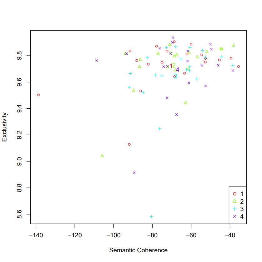
- Model selection for a fixed number of topics
poliblogSelect <- selectModel(out$documents, out$vocab, K = 20, prevalence = ~rating + s(day), max.em.its = 75, data = out$meta, runs = 20, seed = 8458159)
selectModel() first establishes a network (net) for running the model, and runs all models (less than 10 times) E step and M step in turn, discarding the models with low likelihood, and then only runs the top 20% of the models with high likelihood until convergence or the maximum number of iterations (max.em.its) is reached
Select the appropriate model through the semantic consistency and exclusivity displayed by the plotModels() function. The larger the semcooh and exclude, the better the model
# Draw the average score of the graph, and use different legends for each model
plotModels(poliblogSelect, pch=c(1,2,3,4), legend.position="bottomright")
# Select model 3
selectedmodel <- poliblogSelect$runout[[3]]
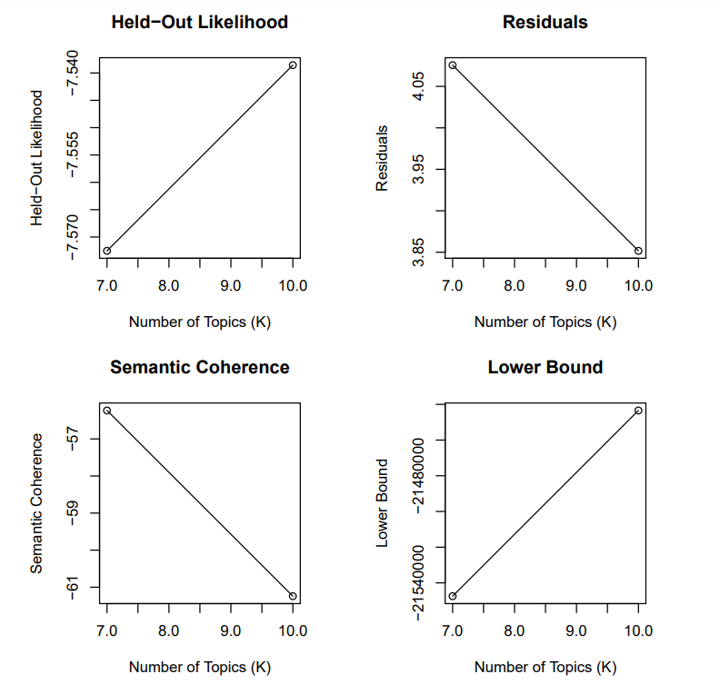
- Model search across numbers of topics
storage <- searchK(out$documents, out$vocab, K = c(7, 10), prevalence = ~rating + s(day), data = meta)

# Visually select the number of topics with the help of chart visualization
pdf("stm-plot-ntopics.pdf")
plot(storage)
dev.off()

# Select the number of topics with actual data
t <- storage$out[[1]]
t <- storage$out[[2]]
Compare the number of two or more topics, and determine the appropriate number of topics by comparing semantic coherence SemCoh and exclusive Exl
3.5 Understand: Interpreting the STM by plotting and inspecting results
After selecting the model, the results of the model are displayed through some functions provided in the stm package. In order to be consistent with the original paper, the initial model poliblogPrevFit is used as a parameter instead of SelectModel
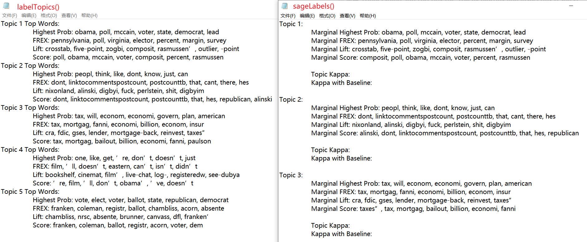
The order of high-frequency words under each topic: labelTopics(), sageLabels()
Both functions output words related to each topic, where sagelabels () is only used for models that contain content covariates. In addition, the result of sageLabels() function is more detailed than that of labelTopics(), and the high-frequency words and other information under all topics are output by default
# labelTopics() Label topics by listing top words for selected topics 1 to 5.
labelTopicsSel <- labelTopics(poliblogPrevFit, c(1:5))
sink("output/labelTopics-selected.txt", append=FALSE, split=TRUE)
print(labelTopicsSel)
sink()

# sageLabels() output is more detailed than labelTopics()
sink("stm-list-sagelabel.txt", append=FALSE, split=TRUE)
print(sageLabels(poliblogPrevFit))
sink()
TODO: the output results of the two functions are different
List documents that are highly relevant to a topic: find hours()
shortdoc <- substr(out$meta$documents, 1, 200)
# The parameter 'texts=shortdoc' indicates that the first 200 characters of each document are output, and n indicates the number of relevant documents output
thoughts1 <- findThoughts(poliblogPrevFit, texts=shortdoc, n=2, topics=1)$docs[[1]]
pdf("findThoughts-T1.pdf")
plotQuote(thoughts1, width=40, main="Topic 1")
dev.off()

# how about more documents for more of these topics?
thoughts6 <- findThoughts(poliblogPrevFit, texts=shortdoc, n=2, topics=6)$docs[[1]]
thoughts18 <- findThoughts(poliblogPrevFit, texts=shortdoc, n=2, topics=18)$docs[[1]]
pdf("stm-plot-find-thoughts.pdf")
# mfrow=c(2, 1) will output the graph to a table with 2 rows and 1 column
par(mfrow = c(2, 1), mar = c(.5, .5, 1, .5))
plotQuote(thoughts6, width=40, main="Topic 6")
plotQuote(thoughts18, width=40, main="Topic 18")
dev.off()

Estimating the relationship between metadata and topic / topic content: estimateEffect
out$meta$rating<-as.factor(out$meta$rating)
# since we're preparing these coVariates by estimating their effects we call these estimated effects 'prep'
# we're estimating Effects across all 20 topics, 1:20. We're using 'rating' and normalized 'day,' using the topic model poliblogPrevFit.
# The meta data file we call meta. We are telling it to generate the model while accounting for all possible uncertainty. Note: when estimating effects of one covariate, others are held at their mean
prep <- estimateEffect(1:20 ~ rating+s(day), poliblogPrevFit, meta=out$meta, uncertainty = "Global")
summary(prep, topics=1)
summary(prep, topics=2)
summary(prep, topics=3)
summary(prep, topics=4)
Uncertainty has three choices: "Global", "Local" and "None". The default is "Global", which will incorporate estimation uncertainty of the topic proportions into the uncertainty estimates using the method of composition If users do not propagate the full amount of uncertainty, e.g., in order to speed up computational time, they can choose uncertainty = “None”, which will generally result in narrower confidence intervals because it will not include the additional estimation uncertainty.
summary(prep, topics=1) output results:
Call:
estimateEffect(formula = 1:20 ~ rating + s(day), stmobj = poliblogPrevFit,
    metadata = meta, uncertainty = "Global")


Topic 1:

Coefficients:
               Estimate Std. Error t value Pr(>|t|)
(Intercept)    0.068408   0.011233   6.090 1.16e-09 ***
ratingLiberal -0.002513   0.002588  -0.971  0.33170
s(day)1       -0.008596   0.021754  -0.395  0.69276
s(day)2       -0.035476   0.012314  -2.881  0.00397 **
s(day)3       -0.002806   0.015696  -0.179  0.85813
s(day)4       -0.030237   0.013056  -2.316  0.02058 *
s(day)5       -0.026256   0.013791  -1.904  0.05695 .
s(day)6       -0.010658   0.013584  -0.785  0.43269
s(day)7       -0.005835   0.014381  -0.406  0.68494
s(day)8        0.041965   0.016056   2.614  0.00897 **
s(day)9       -0.101217   0.016977  -5.962 2.56e-09 ***
s(day)10      -0.024237   0.015679  -1.546  0.12216
---
Signif. codes:  0 '***' 0.001 '**' 0.01 '*' 0.05 '.' 0.1 ' ' 1
3.6 Visualize: Presenting STM results
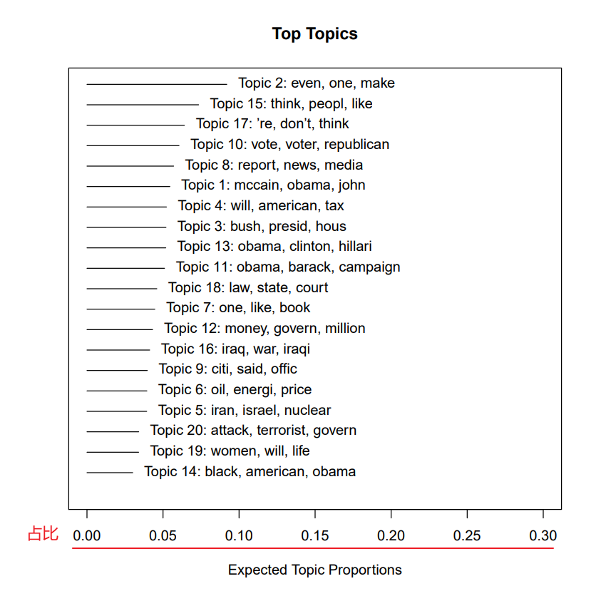
Summary visualization
Subject proportion bar chart
# see PROPORTION OF EACH TOPIC in the entire CORPUS. Just insert your STM output
pdf("top-topic.pdf")
plot(poliblogPrevFit, type = "summary", xlim = c(0, .3))
dev.off()
Metadata/topic relationship visualization
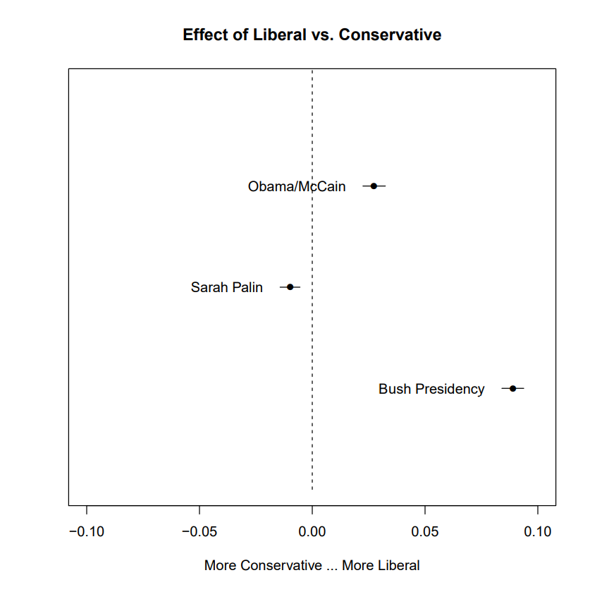
Comparison chart of subject relationship
pdf("stm-plot-topical-prevalence-contrast.pdf")
plot(prep, covariate = "rating", topics = c(6, 13, 18),
     model = poliblogPrevFit, method = "difference",
     cov.value1 = "Liberal", cov.value2 = "Conservative",
     xlab = "More Conservative ... More Liberal",
     main = "Effect of Liberal vs. Conservative",
     xlim = c(-.1, .1), labeltype = "custom",
     custom.labels = c("Obama/McCain", "Sarah Palin", "Bush Presidency"))
dev.off()
Themes 6, 13 and 18 are labeled "Obama/McCain", "Sarah Palin" and "Bush Presidency". The ideology of themes 6 and 13 is neutral, neither conservative nor free, and the ideology of theme 18 is conservative.
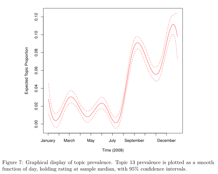
Trend chart of theme over time
pdf("stm-plot-topic-prevalence-with-time.pdf")
plot(prep, "day", method = "continuous", topics = 13,
     model = z, printlegend = FALSE, xaxt = "n", xlab = "Time (2008)")
monthseq <- seq(from = as.Date("2008-01-01"), to = as.Date("2008-12-01"), by = "month")
monthnames <- months(monthseq)
# There were 50 or more warnings (use warnings() to see the first 50)
axis(1, at = as.numeric(monthseq) - min(as.numeric(monthseq)), labels = monthnames)
dev.off()
The operation reports an error, but the following pictures can be output for unknown reasons
topic content
Displays which words in a topic are more closely related to one variable value and another variable value.
# TOPICAL CONTENT.
# STM can plot the influence of covariates included in as a topical content covariate.
# A topical content variable allows for the vocabulary used to talk about a particular
# topic to vary. First, the STM must be fit with a variable specified in the content option.
# Let's do something different. Instead of looking at how prevalent a topic is in a class of documents categorized by meta-data covariate...
# ... let's see how the words of the topic are emphasized differently in documents of each category of the covariate
# First, we we estimate a new stm. It's the same as the old one, including prevalence option, but we add in a content option
poliblogContent <- stm(out$documents, out$vocab, K = 20,
prevalence = ~rating + s(day), content = ~rating,
max.em.its = 75, data = out$meta, init.type = "Spectral")
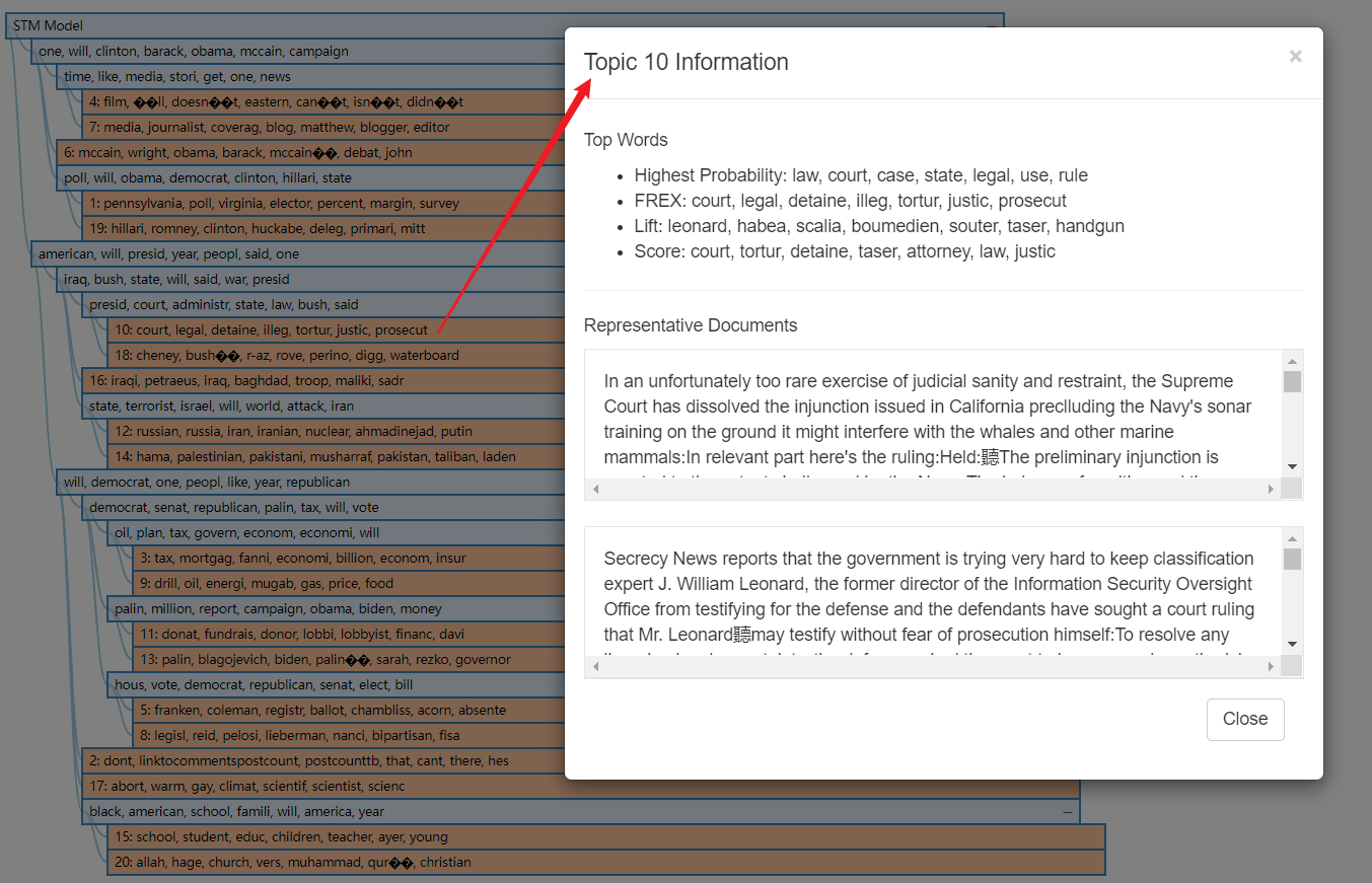
pdf("stm-plot-content-perspectives.pdf")
plot(poliblogContent, type = "perspectives", topics = 10)
dev.off()
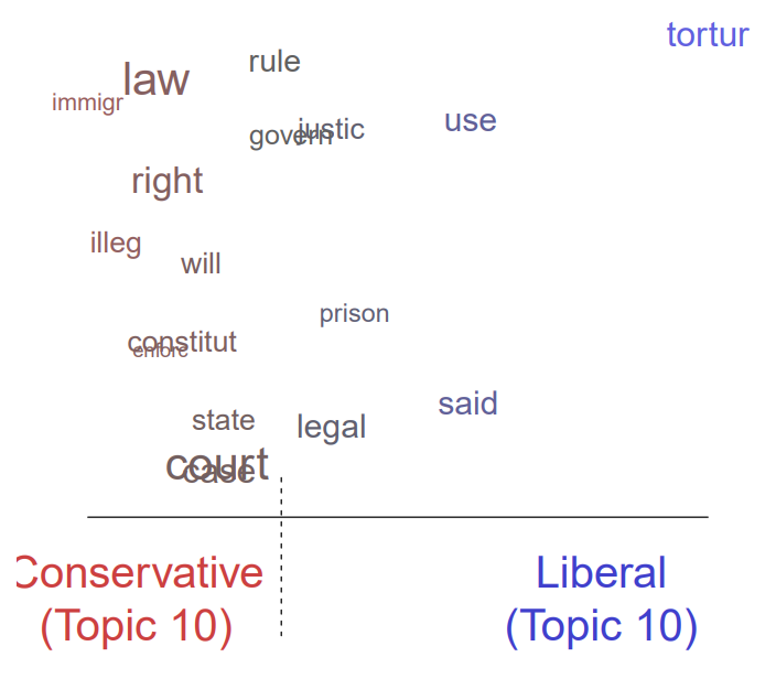
Theme 10 concerns Cuba. Its most commonly used words are "detention, imprisonment, court, illegality, torture, enforcement, Cuba". It shows the different views of liberals and conservatives on the subject. Liberals emphasize "torture", while conservatives emphasize typical court terms such as "illegal" and "law"
Original text: Its top FREX words were "detail, prison, court, illeg, tortur, enforc, Guantanamo"
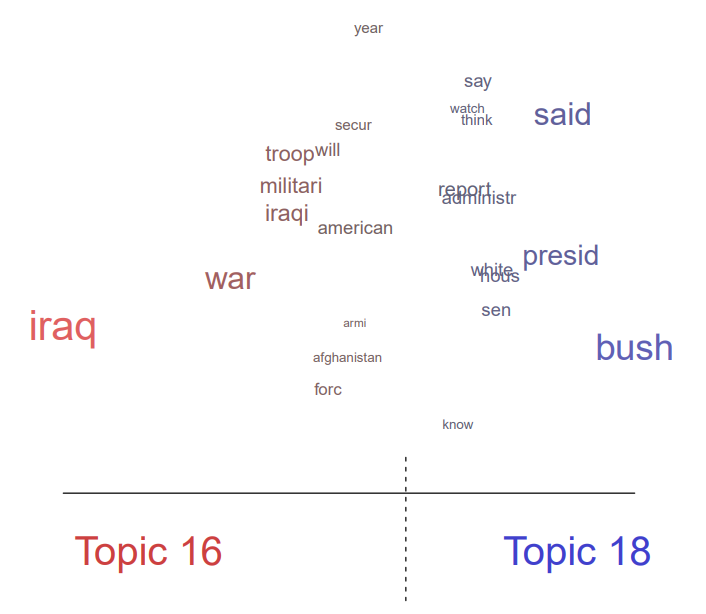
Draw the lexical differences of topic 16
pdf("stm-plot-content-perspectives-16-18.pdf")
plot(poliblogPrevFit, type = "perspectives", topics = c(16, 18))
dev.off()
Plotting covariate interactions
# Interactions between covariates can be examined such that one variable may ??moderate??
# the effect of another variable.
###Interacting covariates. Maybe we have a hypothesis that cities with low $$/capita become more repressive sooner, while cities with higher budgets are more patient
##first, we estimate an STM with the interaction
poliblogInteraction <- stm(out$documents, out$vocab, K = 20,
                           prevalence = ~rating * day, max.em.its = 75,
                           data = out$meta, init.type = "Spectral")
# Prep covariates using the estimateEffect() function, only this time, we include the
# interaction variable. Plot the variables and save as pdf files.
prep <- estimateEffect(c(16) ~ rating * day, poliblogInteraction,
                       metadata = out$meta, uncertainty = "None")
pdf("stm-plot-two-topic-contrast.pdf")
plot(prep, covariate = "day", model = poliblogInteraction,
     method = "continuous", xlab = "Days", moderator = "rating",
     moderator.value = "Liberal", linecol = "blue", ylim = c(0, 0.12),
     printlegend = FALSE)
plot(prep, covariate = "day", model = poliblogInteraction,
     method = "continuous", xlab = "Days", moderator = "rating",
     moderator.value = "Conservative", linecol = "red", add = TRUE,
     printlegend = FALSE)
legend(0, 0.06, c("Liberal", "Conservative"),
       lwd = 2, col = c("blue", "red"))
dev.off()
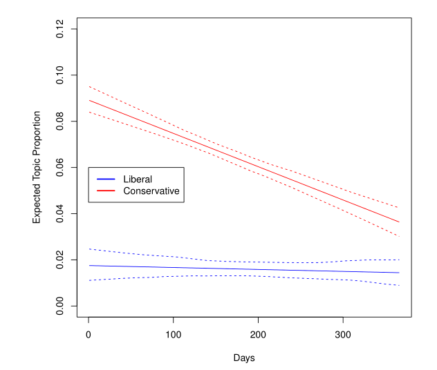
The figure above depicts the relationship between time (the day of blog posting) and score (liberals and conservatives). Topic 16 prevalence was plotted as a linear function of time with a score of 0 (free) or 1 (conservative).
3.7 Extend: Additional tools for interpretation and visualization
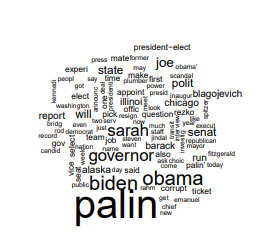
Draw word cloud
pdf("stm-plot-wordcloud.pdf")
cloud(poliblogPrevFit, topic = 13, scale = c(2, 0.25))
dev.off()
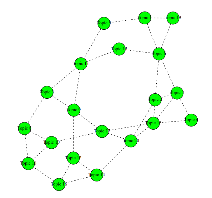
Topic relevance
# topicCorr().
# STM permits correlations between topics. Positive correlations between topics indicate
# that both topics are likely to be discussed within a document. A graphical network
# display shows how closely related topics are to one another (i.e., how likely they are
# to appear in the same document). This function requires 'igraph' package.
# see GRAPHICAL NETWORK DISPLAY of how closely related topics are to one another, (i.e., how likely they are to appear in the same document) Requires 'igraph' package
mod.out.corr <- topicCorr(poliblogPrevFit)
pdf("stm-plot-topic-correlations.pdf")
plot(mod.out.corr)
dev.off()
stmCorrViz
stmCorrViz package A different d3 visualization environment is provided, which focuses on grouping topics using hierarchical clustering method to visualize topic relevance.
There is a problem of garbled code
# The stmCorrViz() function generates an interactive visualisation of topic hierarchy/correlations in a structural topicl model. The package performs a hierarchical
# clustering of topics that are then exported to a JSON object and visualised using D3.
# corrViz <- stmCorrViz(poliblogPrevFit, "stm-interactive-correlation.html", documents_raw=data$documents, documents_matrix=out$documents)

stmCorrViz(poliblogPrevFit, "stm-interactive-correlation.html",
           documents_raw=data$documents, documents_matrix=out$documents)
4 Changing basic estimation defaults
This section explains how to change the default settings in the estimation command of the stm package
Firstly, it discusses how to choose among different methods of initializing model parameters, then discusses how to set and evaluate convergence criteria, and then describes a method to accelerate convergence when analyzing documents containing tens of thousands or more. Finally, it discusses some changes of content covariate model, which allow users to control the complexity of the model.
problem
ems. What is the difference between its and run? ems. The algebra of each iteration, run=20?
How to determine the appropriate number of topics according to the four figures in 3.4-3?
supplement
In the Ingest section, the author mentioned other quanteda packages for text processing, which can easily import text and related metadata, prepare the text to be processed, and convert the document into a document term matrix. Another package, readtext, contains very flexible tools for reading a variety of text formats, such as plain text, XML and JSON, from which you can easily create a corpus.
To read data from other text processing programs, you can use txtorg, which can create three independent files: a metadata file, a verbal file, and a file with the original documents. The default export format is lda-c spark matrix format. You can use readcorps() to set "ldac"option to read
Thesis: stm: An R Package for Structural Topic Models (harvard.edu)
Reference article: R software STM package practice - BiliBili (bilibilibili. Com)
Relevant github warehouses:
JvH13/FF-STM: Web Appendix - Methodology for Structural Topic Modeling (github.com)
dondealban/learning-stm: Learning structural topic modeling using the stm R package. (github.com)
or Structural Topic Models (harvard.edu)](https://scholar.harvard.edu/files/dtingley/files/jss-stm.pdf)
Reference article: R software STM package practice - BiliBili (bilibilibili. Com)
Relevant github warehouses:
JvH13/FF-STM: Web Appendix - Methodology for Structural Topic Modeling (github.com)
dondealban/learning-stm: Learning structural topic modeling using the stm R package. (github.com)
bstewart/stm: An R Package for the Structural Topic Model (github.com)