Today, I'm going to take a simple note of mobilenet. I'm afraid I'll forget the relevant contents of mobilenet. First of all, we need to know that mobilenet is a model framework that can be used on embedded devices. Therefore, its biggest advantage is that it has less parameters, and we still need to ensure that the accuracy of computer vision related tasks cannot be reduced too low. Here are the versions of mobilenet.
Network structure diagram of mobilenetv1
For mobilenetv1, the biggest advantage or improvement is to select the deep separable convolution block to reduce the parameters of general convolution, which can be seen from the following figure. (the source of the picture is the watermark. You can watch the big guy's bilibili bili video. It's great!)
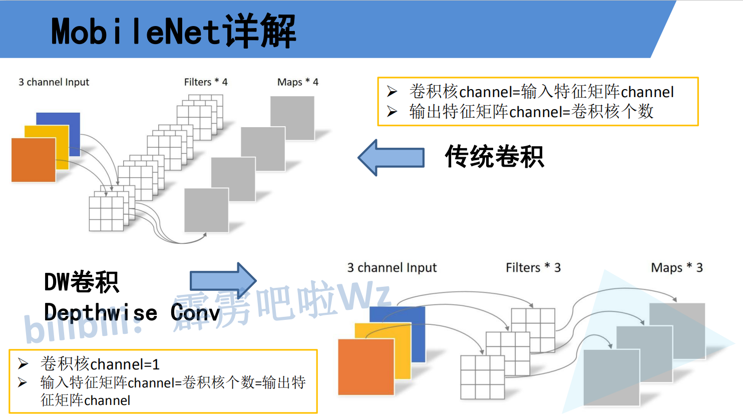
For the traditional convolution mechanism: assuming that the input is a 3x3xc dimension feature map, the convolution is carried out through the 3x3xd convolution block to obtain a 1x1xd special diagnosis map, then the amount of calculation is 3x3xcxdx3x3=81cd
For the deep separable convolution, assuming that the input is a 3x3xc dimension feature map, first perform the deep separable convolution through 3x3xc, that is, convolute each channel to obtain a 1x1xc feature map with a calculation amount of 1x1x3x3xc. The result of convolution through a 1x1xd convolution block is 1x1xd with a calculation amount of 1x1xdx1xc, Then the total calculation amount is 1x1x3xc + 1x1xdx1xc = 9C + CD
By comparing up and down, we can clearly see the gap.
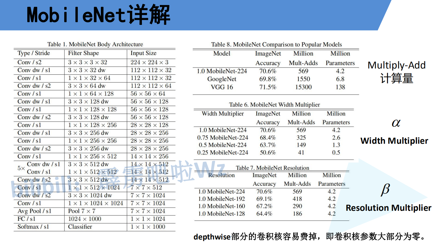
The following is the overall architecture of mobilenetv1. In fact, the original paper also proposed two super parameters, one is α One is β. α The parameter is a magnification factor, which is used to adjust the number of convolution cores. The number of convolution cores is the number of channels passing through 1x1xd convolution blocks after each deep separable convolution. I hope you can understand, β It is the image size parameter that controls the input network, but the depth separable convolution also has the disadvantage shown in the figure below, that is, it is easy to make the convolution kernel parameter become 0 Only then will the mobilenetv2 model appear.
Network structure diagram of mobilenetv2
The following is the block of mobilenetv2, which can be roughly seen as a residual block. Yes, it is so simple. It inherits the deep separable convolution of mobilenetv1, and then makes an innovation, that is, increasing the number of channels first and then decreasing the number of channels. Why do you do this? Because the paper says, Activating the function relu will cause more information loss for low-dimensional features and less loss for high-dimensional features, so there is this innovation. The overall step is to increase the dimension through general convolution, then operate through deep separable convolution, then reduce the dimension through general convolution, and finally add the residuals (the size of the characteristic image must be the same, I believe you know this). See the code for details For the general residual block, it is 1x1 convolution dimension reduction - > 3x3 convolution - > 1x1 convolution dimension increase. This is the difference between the two.
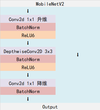
mobilenetv2's block
class InvertedResidual(nn.Module):
def __init__(self, inp, oup, stride, expand_ratio):
super(InvertedResidual, self).__init__()
self.stride = stride
assert stride in [1, 2]#Stripe = 2 is the down sampling operation.
hidden_dim = int(round(inp * expand_ratio))
self.use_res_connect = self.stride == 1 and inp == oup,Judge whether the number of output channels is the same as that of output channels. If you don't want to add, you're down sampling.
layers = []
if expand_ratio != 1:
layers.append(ConvBNReLU(inp, hidden_dim, kernel_size=1))
layers.extend([
ConvBNReLU(hidden_dim, hidden_dim, stride=stride, groups=hidden_dim),
nn.Conv2d(hidden_dim, oup, 1, 1, 0, bias=False),
nn.BatchNorm2d(oup),
])
self.conv = nn.Sequential(*layers)
def forward(self, x):
if self.use_res_connect:
return x + self.conv(x)#This is the addition, not the splicing of the number of channels. You should understand it
else:
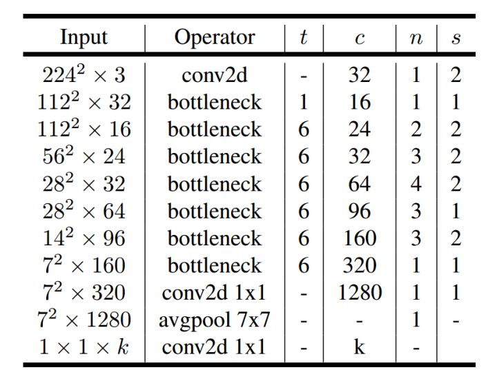
return self.conv(x)The following is the overall structure of mobilenetv2. The structure diagram is interpreted as follows:
Input represents the size of the input characteristic graph, starting from the second one, and also represents the output result of the previous convolution block (I believe you can understand this)
The Operator represents the execution code block. Except for the first and last three, they are the final convolution blocks to form mobilenetv2, which is as shown in the above code.
T represents the expansion factor, that is, in each block, the number of ascending channels is t times the number of input channels.
n represents how many times the block needs to be executed
S represents the step size , but it should be noted here that as long as the step size is greater than 1, it is for the first block. For example, when n=2, s=2, then only the strip of the first block is 2 and the s of the other block is 1
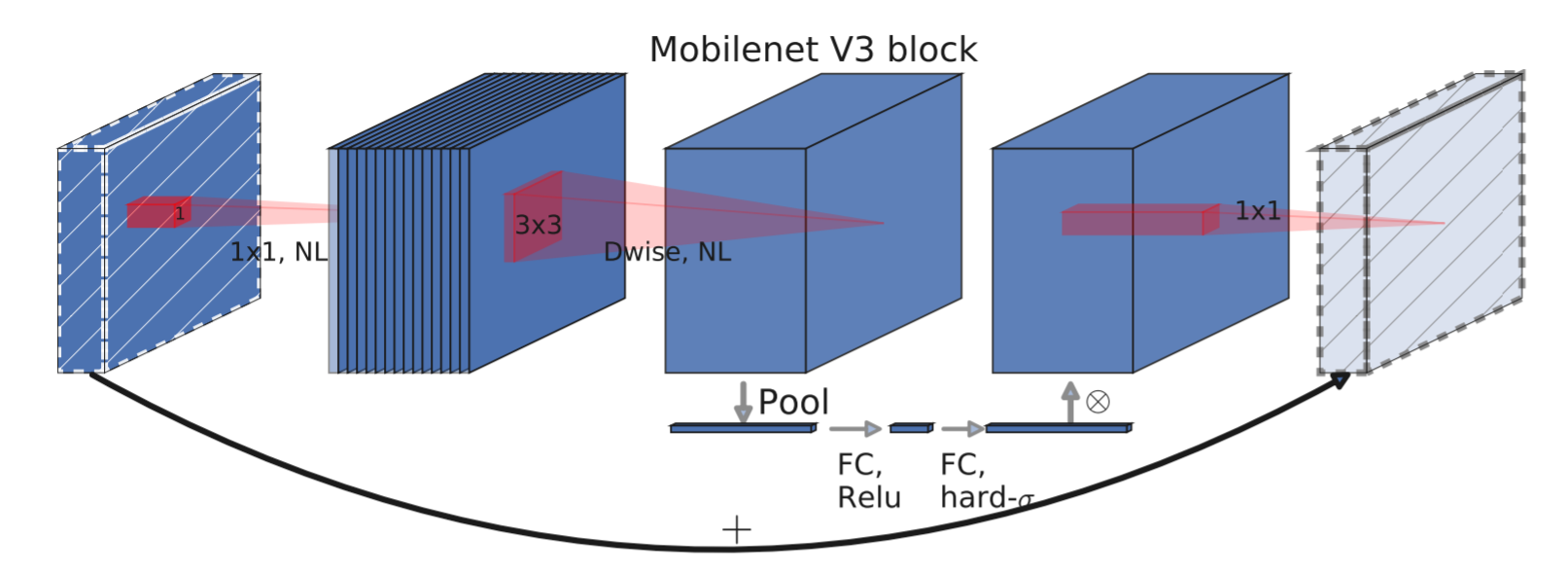
Network structure diagram of mobilenetv3
For mobilenetv3, another big improvement is the application of channel attention mechanism. It is to pool the input feature map into 1x1xc size, and then flatten ----- > full connection -------- > full connection -------- > sigmoid() -------- > to get the size of 1x1xc, and then multiply it with the input feature map on the channel, so as to achieve the function of channel attention mechanism. See the following code for details.
mobilenetv3's block
class InvertedResidual(nn.Module):
    def __init__(self, inp, hidden_dim, oup, kernel_size, stride, use_se, use_hs):
        super(InvertedResidual, self).__init__()
        assert stride in [1, 2]

        self.identity = stride == 1 and inp == oup

        if inp == hidden_dim:
            self.conv = nn.Sequential(
                # dw
                nn.Conv2d(hidden_dim, hidden_dim, kernel_size, stride, (kernel_size - 1) // 2, groups=hidden_dim, bias=False),
                nn.BatchNorm2d(hidden_dim),
                h_swish() if use_hs else nn.ReLU(inplace=True),
                # Squeeze-and-Excite
                SELayer(hidden_dim) if use_se else nn.Identity(),
                # pw-linear
                nn.Conv2d(hidden_dim, oup, 1, 1, 0, bias=False),
                nn.BatchNorm2d(oup),
            )
        else:
            self.conv = nn.Sequential(
                # pw
                nn.Conv2d(inp, hidden_dim, 1, 1, 0, bias=False),
                nn.BatchNorm2d(hidden_dim),
                h_swish() if use_hs else nn.ReLU(inplace=True),
                # dw
                nn.Conv2d(hidden_dim, hidden_dim, kernel_size, stride, (kernel_size - 1) // 2, groups=hidden_dim, bias=False),
                nn.BatchNorm2d(hidden_dim),
                # Squeeze-and-Excite
                SELayer(hidden_dim) if use_se else nn.Identity(),
                h_swish() if use_hs else nn.ReLU(inplace=True),
                # pw-linear
                nn.Conv2d(hidden_dim, oup, 1, 1, 0, bias=False),
                nn.BatchNorm2d(oup),
            )

    def forward(self, x):
        if self.identity:
            return x + self.conv(x)
        else:
            return self.conv(x)
The channel attention mechanism code is shown in the figure below:
# class SqueezeExcitation(nn.Module):#Attention mechanism
#     def __init__(self, input_c: int, squeeze_factor: int = 4):
#         super(SqueezeExcitation, self).__init__()
#         squeeze_c = _make_divisible(input_c // squeeze_factor, 8) # this function is to change the number of input channels into a multiple of 8 nearest to 8. This is a self-made function.
#         self.fc1 = nn.Conv2d(input_c, squeeze_c, 1)
#         self.fc2 = nn.Conv2d(squeeze_c, input_c, 1)
#
#     def forward(self, x):
#         scale = F.adaptive_avg_pool2d(x, output_size=(1, 1))
#         scale = self.fc1(scale)
#         scale = F.relu(scale, inplace=True)
#         scale = self.fc2(scale)
#         scale = F.hardsigmoid(scale, inplace=True)
#         return scale * x
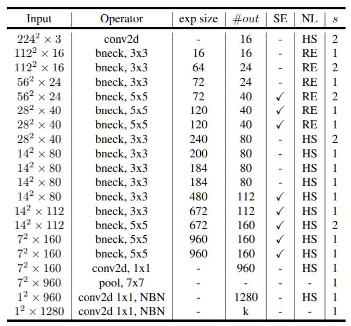
The following is the model architecture diagram of mobilenetv3, which is similar to that of v2, with the addition of Se (whether to use the attention mechanism module) and NL (the use of three activation functions), exp_size is also an expansion factor, but this is the result of expansion, not a multiple.
Finally, the code of this blog comes from: