Steel defect detection project case
1, Project introduction
This project comes from Kaggle's last project Steel surface defect detection competition , this is also a very good case of applying deep learning to traditional industrial material testing. This project will use Baidu PaddlePaddle. PaddleX Develop the deep learning algorithm suite, analyze the whole process and the whole implementation process.
Steel is one of the most important building materials in modern times. Rigid structure buildings can resist natural and man-made wear, which makes this material everywhere in the world. In all steel processing links, the production process of flat steel is particularly fine. From heating, rolling, drying and cutting, several machines need to work together. One important link is to use the images captured by high-definition cameras to automatically detect the defects of steel in the processing link. The steel defect competition held in Kaggle hopes that all participants can use machine learning to improve the accuracy of steel plate surface defect detection algorithm and improve the automation of steel production.
2, Data set analysis
The main purpose of this competition is to locate and classify the surface defects of steel plate, which belongs to the problem of semantic segmentation. The corresponding data set can be from Kaggle competition official website Download, or from ai studio Download. After downloading, it contains two image folders and two annotation files:
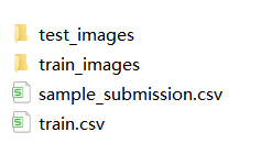
Corresponding to the following:
- train_images: this folder stores training images
- test_images: this folder stores test images
- train.csv: this file stores defect labels of training images. There are 4 types of defects, ClassId = [1, 2, 3, 4]
- sample_submission.csv: this file is an example of an uploaded file. Each ImageID should have 4 lines, and each line corresponds to a type of defect
For the competition, the first thing we need to do after we get the data is to analyze the data set. Let's analyze this data set step by step according to text and image.
2.1 reading and analyzing text data
Suppose that the downloaded data set is placed in a folder named severstal, and the csv text data is read first
import pandas as pd
from collections import defaultdict

train_df = pd.read_csv("severstal/train.csv")
sample_df = pd.read_csv("severstal/sample_submission.csv")
Take a preliminary look at the data inside
print(train_df.head())
print('\r\n')
print(sample_df.head())
The results are as follows:
   ImageId_ClassId                                      EncodedPixels
0  0002cc93b.jpg_1  29102 12 29346 24 29602 24 29858 24 30114 24 3...
1  0002cc93b.jpg_2                                                NaN
2  0002cc93b.jpg_3                                                NaN
3  0002cc93b.jpg_4                                                NaN
4  00031f466.jpg_1                                                NaN

   ImageId_ClassId EncodedPixels
0  004f40c73.jpg_1           1 1
1  004f40c73.jpg_2           1 1
2  004f40c73.jpg_3           1 1
3  004f40c73.jpg_4           1 1
4  006f39c41.jpg_1           1 1
Note the annotation form of data. There are two columns in total: column 1: ImageId_ClassId (picture number + class number); The second example EncodedPixels (image labels). Note that this image tag is different from what we usually encounter. The usual is a mask gray image, which is filled with many numbers and the background is 0. However, in order to reduce the data, it uses the pixel "column position length" format. for instance:
We take an image (h,w) flatten (note that it is not by row but by column), 29102 12 29346 24 29602 24 indicates that the 12 lengths from the 29102 pixel position are non background, and so on. This is equivalent to drawing a vertical line on each image.
Next, count whether there are defects and the number of images of each type of defects:
class_dict = defaultdict(int)
kind_class_dict = defaultdict(int)
no_defects_num = 0
defects_num = 0

for col in range(0, len(train_df), 4):
    img_names = [str(i).split("_")[0] for i in train_df.iloc[col:col+4, 0].values]
    if not (img_names[0] == img_names[1] == img_names[2] == img_names[3]):
        raise ValueError

    labels = train_df.iloc[col:col+4, 1]
    if labels.isna().all():
        no_defects_num += 1
    else:
        defects_num += 1

    kind_class_dict[sum(labels.isna().values == False)] += 1

    for idx, label in enumerate(labels.isna().values.tolist()):
        if label == False:
            class_dict[idx+1] += 1
Number of images with and without defects output
print("Number of defect free steel plates: {}".format(no_defects_num))
print("Number of defective steel plates: {}".format(defects_num))
The output result is:
Number of defect free steel plates: 5902
 Number of defective steel plates: 6666
Next, classify and count the defective images:
import seaborn as sns
import matplotlib.pyplot as plt

fig, ax = plt.subplots()
sns.barplot(x=list(class_dict.keys()), y=list(class_dict.values()), ax=ax)
ax.set_title("the number of images for each class")
ax.set_xlabel("class")
plt.show()
print(class_dict)
The output results are as follows:
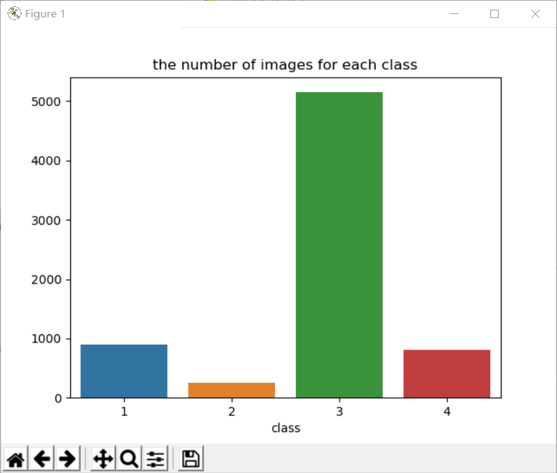
defaultdict(<class 'int'>, {1: 897, 3: 5150, 4: 801, 2: 247})
There are two conclusions here:
(1) The number of defective and non defective images is roughly the same;
(2) The category of defects is unbalanced.
Next, count the number of possible defect types in an image:
fig, ax = plt.subplots()
sns.barplot(x=list(kind_class_dict.keys()), y=list(kind_class_dict.values()), ax=ax)
ax.set_title("Number of classes included in each image");
ax.set_xlabel("number of classes in the image")
plt.show()
print(kind_class_dict)
The output results are as follows:
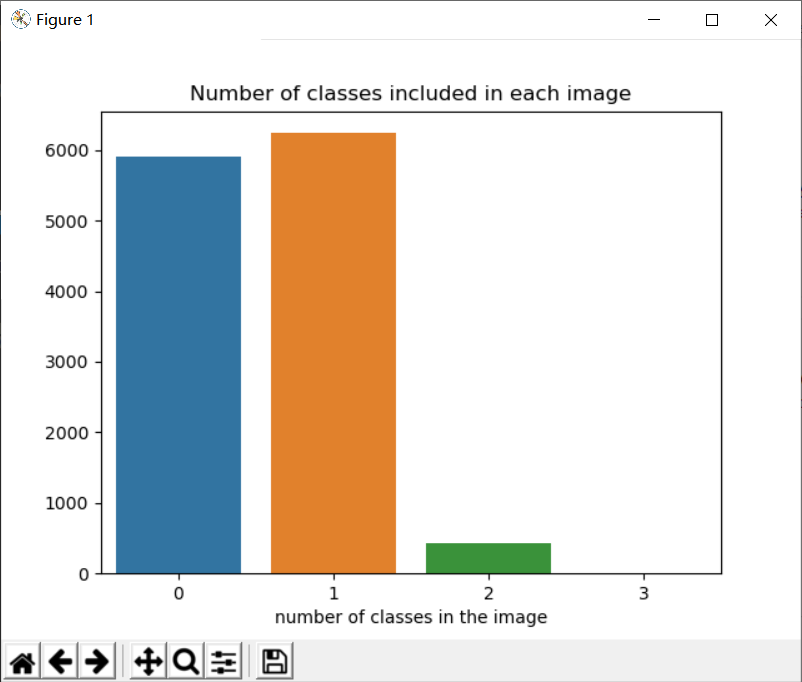
defaultdict(<class 'int'>, {1: 6239, 0: 5902, 2: 425, 3: 2})
The conclusion of this step is:
Most images have no defects or contain only one defect, and no one image in the training set will contain four defects at the same time.
2.2 reading and analyzing image data
Reading training set image data
from collections import defaultdict
from pathlib import Path
from PIL import Image

train_size_dict = defaultdict(int)
train_path = Path("severstal/train_images/")
for img_name in train_path.iterdir():
    img = Image.open(img_name)
    train_size_dict[img.size] += 1
On the one hand, the above code checks whether the size of all images in the training set is consistent, and also checks whether each image format is normal and can be opened normally.
Check the size and number of images in the training set
print(train_size_dict)
Output results:
defaultdict(<class 'int'>, {(1600, 256): 12568})
It can be seen that the size of images in the training set is 1600 times 256, a total of 12568. All images are the same size.
Next, read the test set image data:
test_size_dict = defaultdict(int)
test_path = Path("severstal/test_images/")

for img_name in test_path.iterdir():
    img = Image.open(img_name)
    test_size_dict[img.size] += 1

print(test_size_dict)
Output results:
defaultdict(<class 'int'>, {(1600, 256): 1801})
The images in the test set are 1600 times 256, a total of 1801.
2.3 visual dataset
First read the csv text data
import numpy as np
import pandas as pd
import matplotlib.pyplot as plt
from pathlib import Path
import cv2

train_df = pd.read_csv("severstal/train.csv")
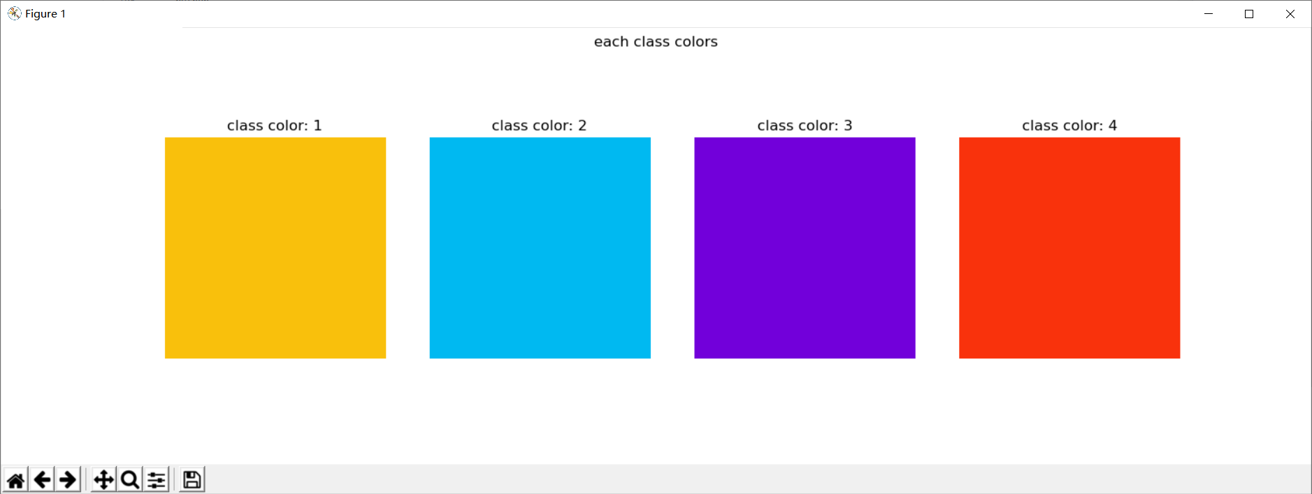
To facilitate visualization, we set color display for different defect categories:
palet = [(249, 192, 12), (0, 185, 241), (114, 0, 218), (249,50,12)]
fig, ax = plt.subplots(1, 4, figsize=(15, 5))
for i in range(4):
    ax[i].axis('off')
    ax[i].imshow(np.ones((50, 50, 3), dtype=np.uint8) * palet[i])
    ax[i].set_title("class color: {}".format(i+1))

fig.suptitle("each class colors")
plt.show()
The output is as follows:
Next, classify different defect identifications:
idx_no_defect = []
idx_class_1 = []
idx_class_2 = []
idx_class_3 = []
idx_class_4 = []
idx_class_multi = []
idx_class_triple = []

for col in range(0, len(train_df), 4):
    img_names = [str(i).split("_")[0] for i in train_df.iloc[col:col+4, 0].values]
    if not (img_names[0] == img_names[1] == img_names[2] == img_names[3]):
        raise ValueError

    labels = train_df.iloc[col:col+4, 1]
    if labels.isna().all():
        idx_no_defect.append(col)
    elif (labels.isna() == [False, True, True, True]).all():
        idx_class_1.append(col)
    elif (labels.isna() == [True, False, True, True]).all():
        idx_class_2.append(col)
    elif (labels.isna() == [True, True, False, True]).all():
        idx_class_3.append(col)
    elif (labels.isna() == [True, True, True, False]).all():
        idx_class_4.append(col)
    elif labels.isna().sum() == 1:
        idx_class_triple.append(col)
    else:
        idx_class_multi.append(col)

train_path = Path("severstal/train_images/")
Next, create a visual annotation function:
def name_and_mask(start_idx):
    col = start_idx
    img_names = [str(i).split("_")[0] for i in train_df.iloc[col:col+4, 0].values]
    if not (img_names[0] == img_names[1] == img_names[2] == img_names[3]):
        raise ValueError

    labels = train_df.iloc[col:col+4, 1]
    mask = np.zeros((256, 1600, 4), dtype=np.uint8)

    for idx, label in enumerate(labels.values):
        if label is not np.nan:
            mask_label = np.zeros(1600*256, dtype=np.uint8)
            label = label.split(" ")
            positions = map(int, label[0::2])
            length = map(int, label[1::2])
            for pos, le in zip(positions, length):
                mask_label[pos-1:pos+le-1] = 1
            mask[:, :, idx] = mask_label.reshape(256, 1600, order='F')  #Value reshape by column

    return img_names[0], mask

def show_mask_image(col):
    name, mask = name_and_mask(col)
    img = cv2.imread(str(train_path / name))
    fig, ax = plt.subplots(figsize=(15, 15))
    for ch in range(4):
        contours, _ = cv2.findContours(mask[:, :, ch], cv2.RETR_LIST, cv2.CHAIN_APPROX_NONE)
        for i in range(0, len(contours)):
            cv2.polylines(img, contours[i], True, palet[ch], 2)

    ax.set_title(name)
    ax.imshow(img)
    plt.show()
Next, show 5 flawless images:
for idx in idx_no_defect[:5]:
    show_mask_image(idx)
The output results are as follows:
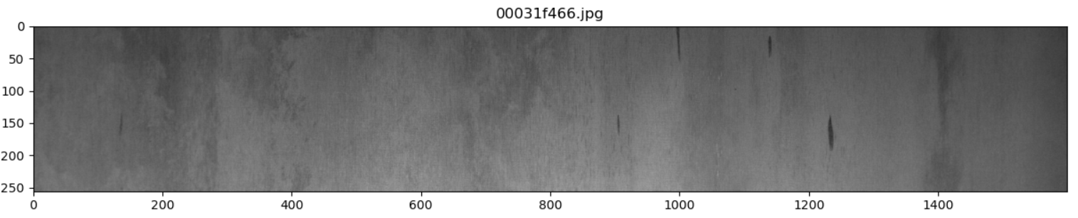
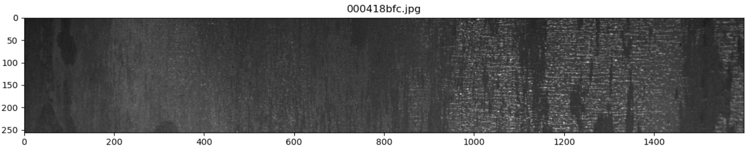
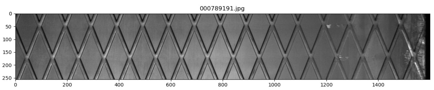
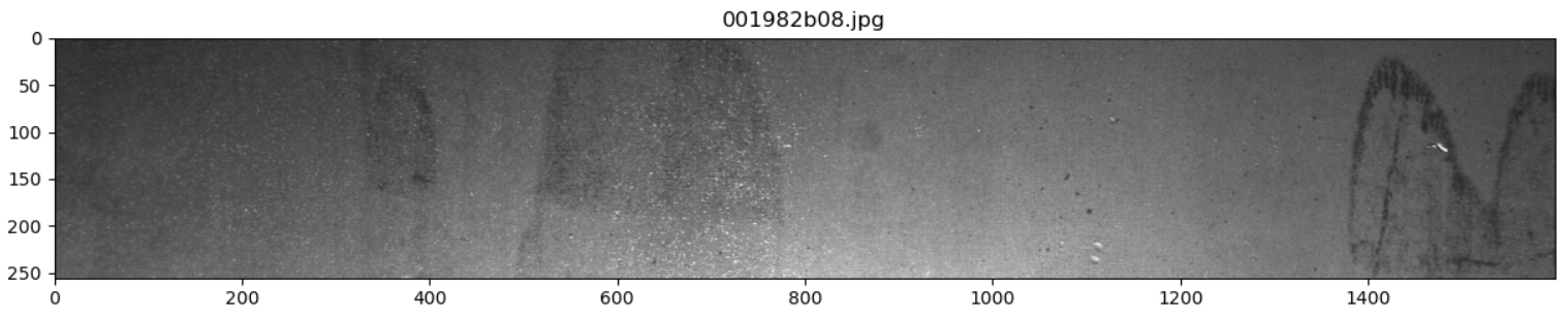
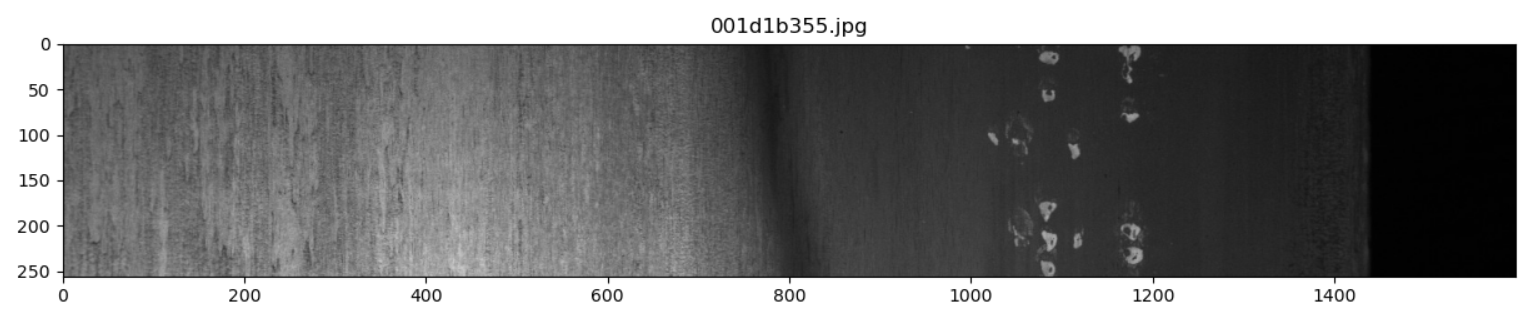
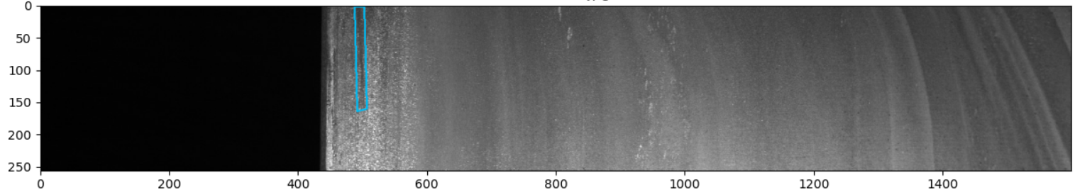
Image display of type 1 defects only:
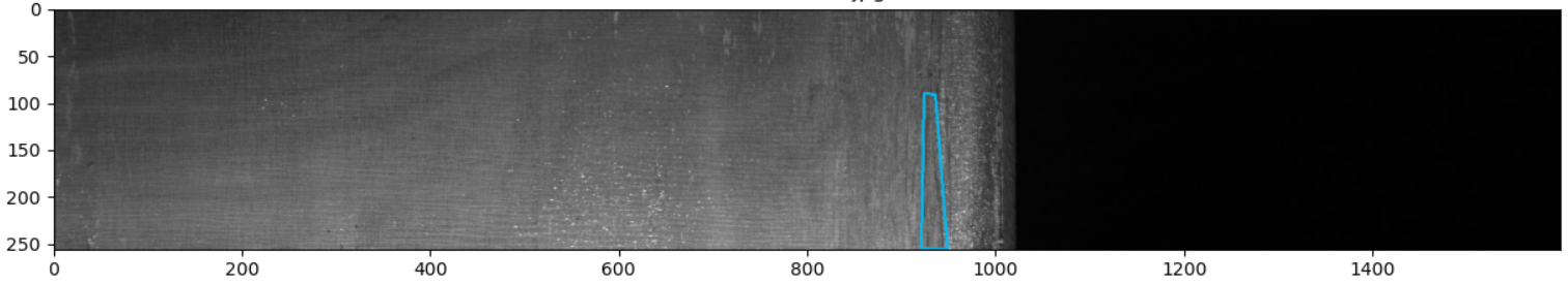
for idx in idx_class_1[:5]:
    show_mask_image(idx)
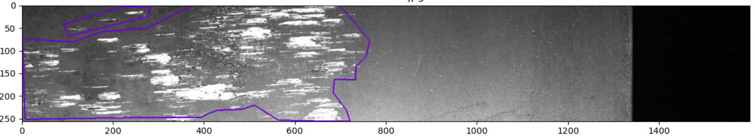
The output results are as follows:
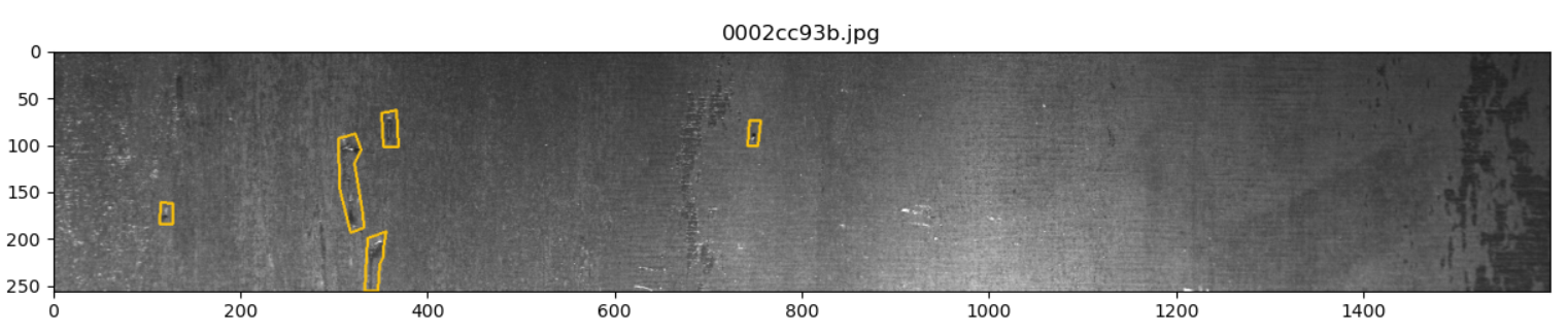
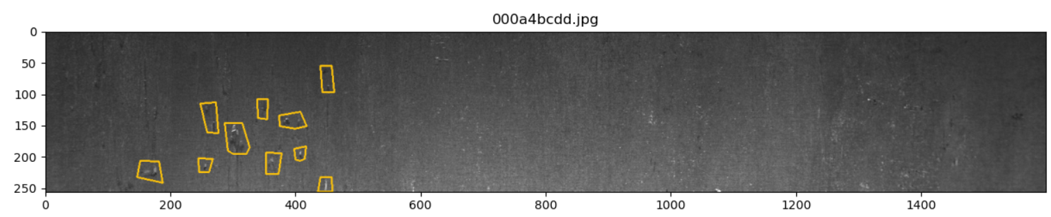
From the image analysis, the first type of defect is mainly the local mixed area of white noise and black noise.
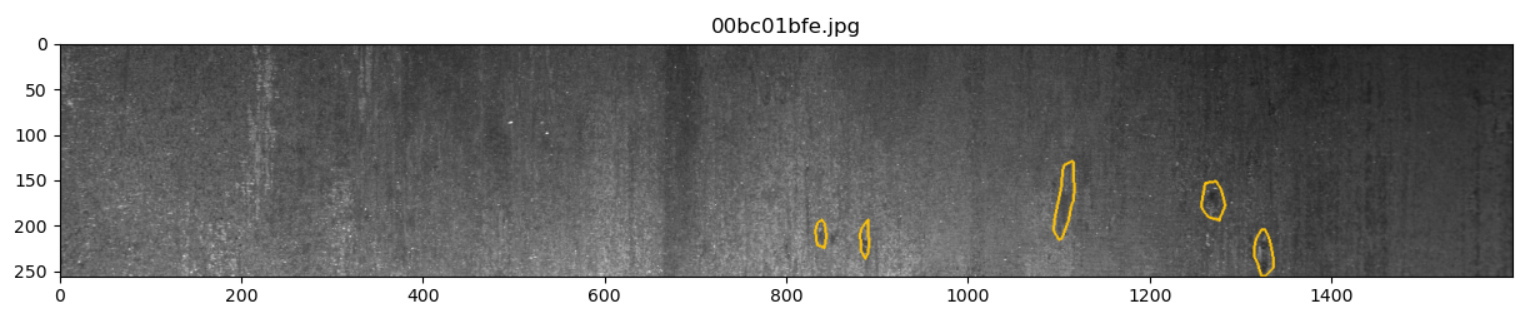
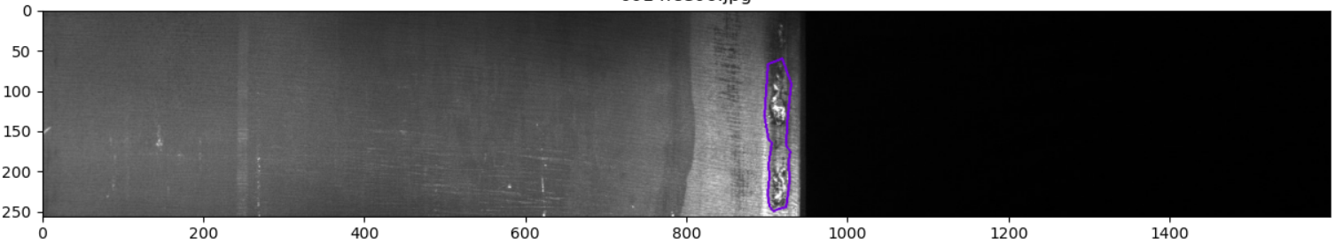
Image display with type 2 defects only:
for idx in idx_class_2[:5]:
    show_mask_image(idx)
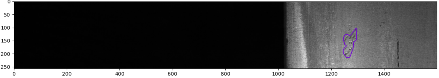
The output results are as follows:
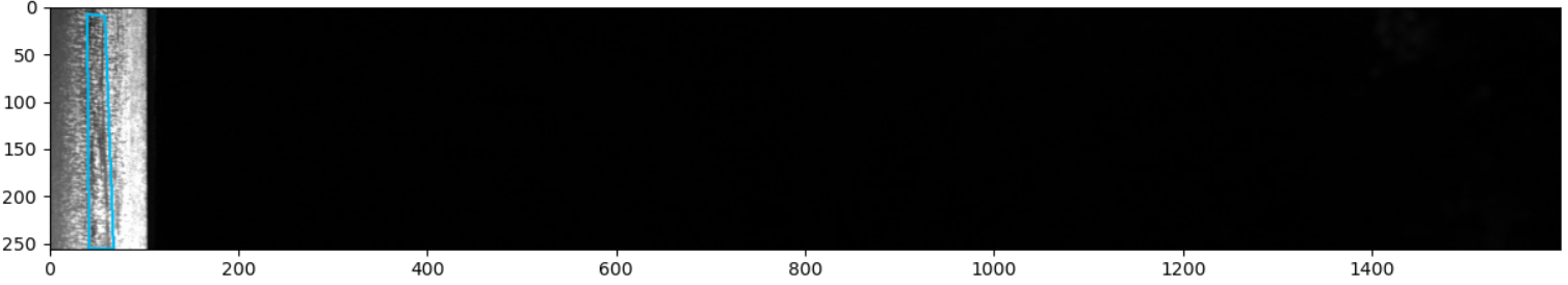
From the image analysis, the second type of defects are mainly vertical black scratches
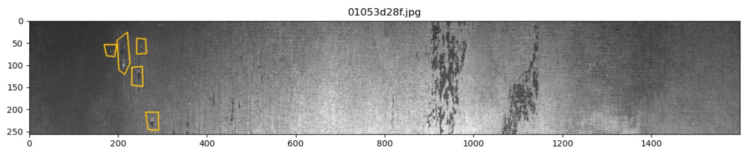
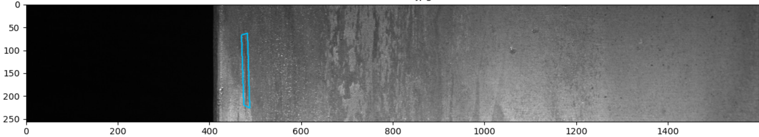
Image display of type 3 defects only:
for idx in idx_class_3[:5]:
    show_mask_image(idx)
The output results are as follows:

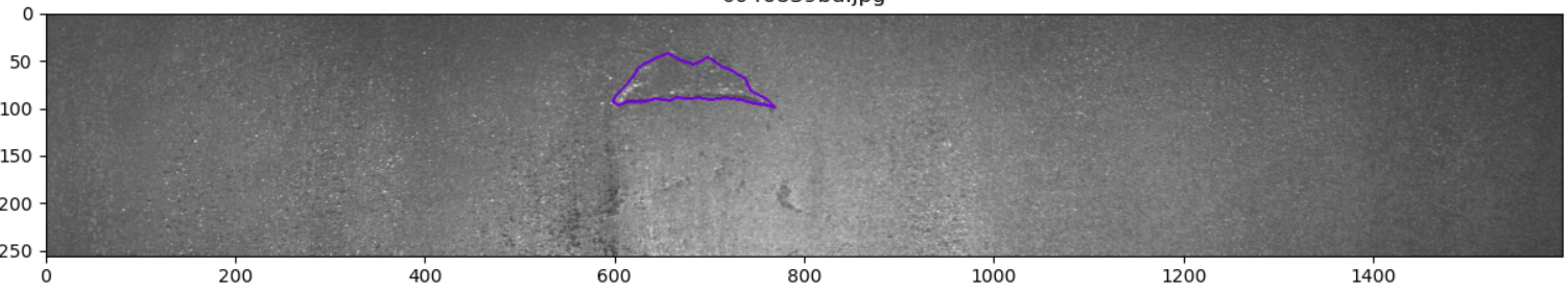


From the image analysis, the types of type 3 defects are relatively diverse, which can also be seen from the proportion of type 3 defects obtained from the previous analysis. In summary, the third type of defect is mainly the patchy area of white noise and white scratches.
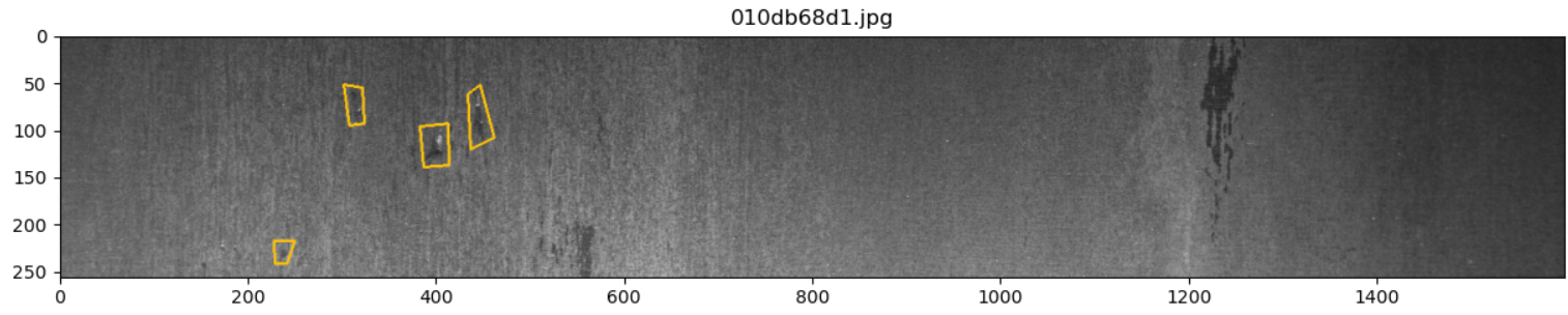
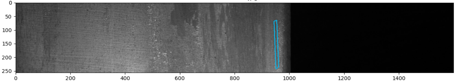
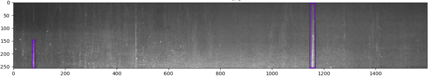
Image display of type 4 defects only:
for idx in idx_class_4[:5]:
    show_mask_image(idx)
The output results are as follows:


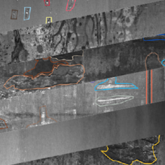
Finally, let's look at the pictures with three defects at the same time:
for idx in idx_class_triple:
    show_mask_image(idx)

The above analysis can help us quickly grasp the basic attributes of data and preliminarily understand the difficulty of the project. In the actual competition, these data analysis is very important. Through these data analysis, mining and sorting into important "clues", and then improving the algorithm model, we can often achieve unexpected good results.
3, Making standard data sets
3.1 format description of paddlex dataset
From the previous data analysis, we can see that each pixel of the steel plate image belongs to only one defect category (or no defect). Since we need to locate the fine area of the steel plate defect, we can regard this task as a semantic segmentation task, that is, judge the defect category of each pixel according to the pixel level accuracy.
Next, we can use semantic segmentation algorithm for training and verification. This project uses Baidu PaddlePaddle PaddleX algorithm suite to train quickly. Paddlex is a full process development tool for the propeller. It integrates all the capabilities required for in-depth learning and development such as the propeller core framework, model library, tools and components, and opens up the whole process of in-depth learning and development. In short, using paddlex has two obvious benefits:
- Fast verification of algorithm model: no algorithm is omnivorous whether it is doing industrial projects or participating in competitions like Kaggle, so we must try many different algorithms. At this time, it is particularly important to quickly verify the effectiveness of algorithm model. For an unknown deep learning task, we don't know what kind of model algorithm to use at the beginning to get a better benchmark value. At this time, we need a algorithm library tool with simple interface switching, fast and convenient implementation and complete algorithm functions to enable us to quickly verify the effectiveness of the model, Here, PaddleX is such a good tool. It contains common and practical deep learning models such as image classification, segmentation and detection, and the interface is highly unified. We can use it to quickly train each model and select a better benchmark value. On this basis, we will optimize the algorithm.
- Rapid model deployment: for real industrial tasks, not only to train a high-precision algorithm model, but also to consider the convenience and effectiveness of deployment. Although many models have high accuracy, due to the very nested dynamic graph model writing method, if they are exported directly or converted to onnx, they often encounter problems. At this time, Algorithm Engineers must modify the model manually, which will greatly increase the difficulty of project development and reduce the efficiency of project development for real projects. The advantage of using PaddleX is that the models in PaddleX have basically been verified, and can be deployed on a variety of platforms, such as C + + reasoning, mobile terminal reasoning, etc. at the same time, it also gives a detailed deployment tutorial. Therefore, choosing PaddleX for real in-depth learning, product development or competition is a good choice.
PaddleX installation method reference Official website . This project is implemented with PaddleX v2.0.0.
In order to use PaddleX for semantic segmentation training, we must first transform the data set format. PaddleX semantic segmentation algorithm requirement Data sets are organized as follows:
The original drawings are placed in the same directory, such as JPEGImages, and the png files with the same name marked are placed in the same directory, such as Annotations. Examples are as follows:
MyDataset/ # Semantic segmentation dataset root directory
|--JPEGImages/ # Directory of original drawing file
|  |--1.jpg
|  |--2.jpg
|  |--...
|  |--...
|
|--Annotations/ # Label the directory where the file is located
|  |--1.png
|  |--2.png
|  |--...
|  |--...
JPEGImages directory stores the original file image (jpg format), and Annotations stores the corresponding annotation file image (PNG format). The annotation image here, such as 1.png, is a single channel image, and the pixel annotation categories need to be incremented from 0. For example, 0, 1, 2 and 3 represent four categories (generally 0 represents background), and the annotation categories can be up to 255 categories (in which the pixel value 255 does not participate in training and evaluation).
3.2 data conversion
The data conversion itself is not difficult. The defect area has been displayed when visualizing the data. Therefore, during data conversion, you only need to fill the gray value corresponding to the defect into the mask.
Will download data set After decompression, place it in the root directory of the current project, and then execute the following code:
python prepare_dataset.py
After execution, a padlex standard dataset named steel will be generated in the current root directory.
After execution, create a label description file under the generated steel folder. The file name is labels.txt, and the content is as follows:
0
1
2
3
4
This file is used to indicate which pixel tag values are currently available (there are 4 defects in this project, and the corresponding tags are 1, 2, 3 and 4. Here, the 0 tag represents the background)
The converted dataset can also be directly from ai studio download.
3.3 data segmentation
During model training, we need to divide the training set, verification set and test set. We can directly use the PaddleX command to randomly divide the data set. In this project, the training set, verification set and test set are divided according to the ratio of 8.5:1:0.5. PaddleX provides a simple and easy-to-use API for users to use directly for data division. The specific commands are as follows:
paddlex --split_dataset --format SEG --dataset_dir steel --val_value 0.1 --test_val 0.05
The status before and after data folder segmentation is as follows:
  steel/                            steel/
  ├── Annotations/      -->         ├── Annotations/
  ├── JPEGImages/                   ├── JPEGImages/
  ├── labels.txt                    ├── labels.txt
                                    ├── test_list.txt
                                    ├── train_list.txt
                                    ├── val_list.txt
Executing the above command line will generate train_list.txt, val_list.txt and test_list.txt under steel to store training sample list, verification sample list and test sample list respectively.
4, Training and verification
PaddleX provides rich visual models and deep labv3, UNET, HRNET and FastSCNN series models in semantic segmentation. In this project, heavyweight HRNET is used as the segmentation model for steel plate defect detection.
4.1 Based on HRNet model
4.2 Based on UNet model
5, Deploy
5.1 model export
After training, the model is saved in the output folder. If you want to use PaddleInference for deployment, you need to export the model into a static diagram. Run the following command to automatically create a folder of information_model in the output folder to store the exported model.
paddlex --export_inference --model_dir=output/hrnet/best_model --save_dir=output/inference_model
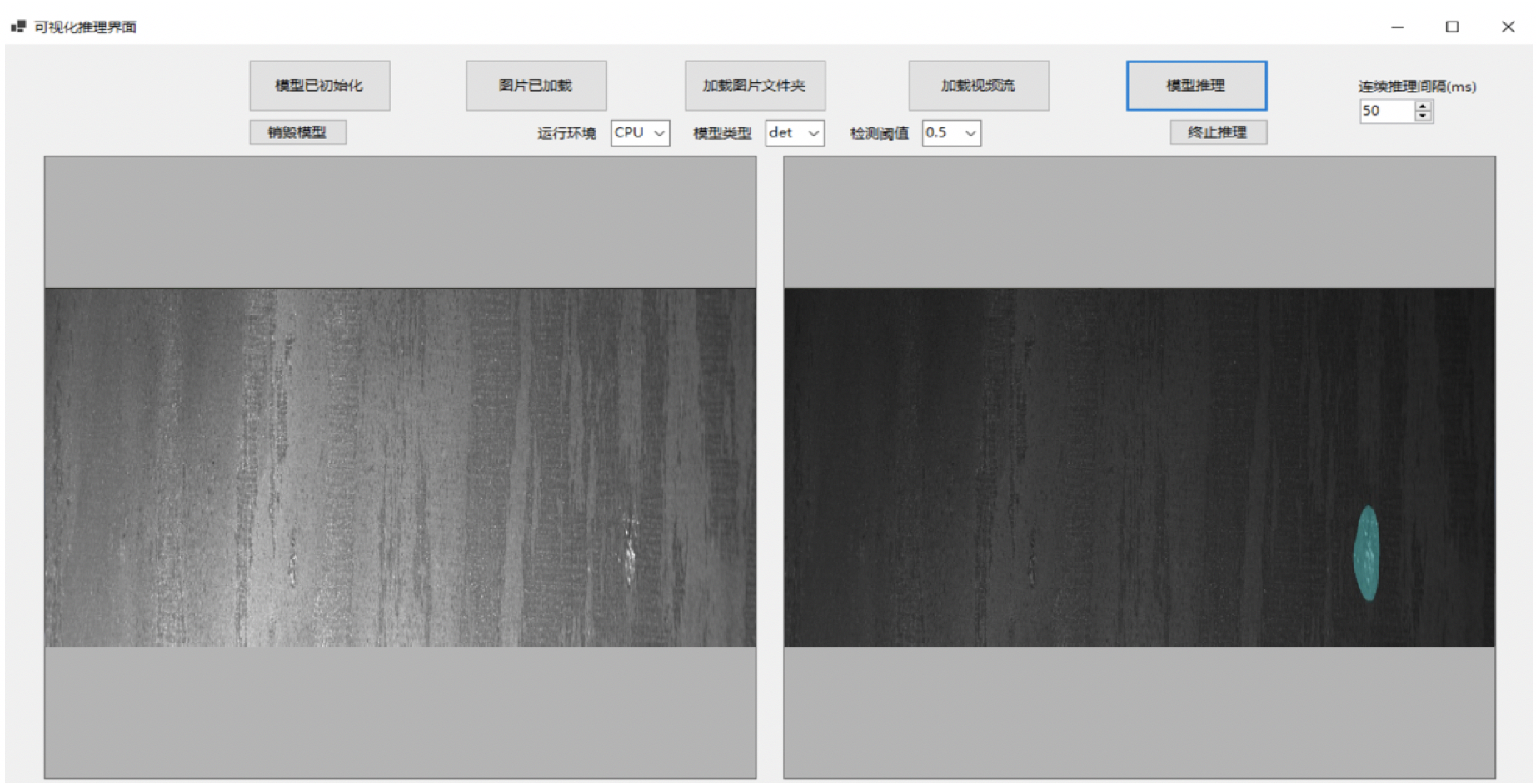
5.2 C# Desktop Deployment
The model deployment adopts the C + + information deployment scheme provided by PaddleX, in which c# deployment is provided Demo , the user can refer to and modify it according to the actual situation.