The three neural networks described above are "series", just the continuous stacking of convolution layers, and the structure is relatively simple. The next two blogs will introduce the "parallel" structure in GoogLeNet and ResNet, which are also the last two neural networks to be introduced before officially entering the target detection algorithm!

1, Introduction

The overall framework of target detection is composed of backbone, neck and head. Therefore, before learning the specific target detection algorithm, it is necessary to understand the common convolutional neural network structure, which is conducive to learning the backbone part of the target detection algorithm later. AlexNet and VGGNet mentioned earlier obtain better training results by increasing the number of network layers, but blindly increasing the number of network layers will cause a waste of computing resources. To increase network complexity, we should consider not only "depth" but also "width". GoogLeNet's practice has inspired a series of network structures behind, so it is necessary to understand.

VGGNet mentioned in the last blog won the runner up in the ImageNet image classification competition in 2014, and the champion is GoogLeNet introduced in this article. GoogLeNet focuses on deepening the network structure, with a total of 22 layers without a full connection layer. At the same time, it introduces a new basic structure - Inception module to increase the width of the network, which is also the core improvement. The original idea of GoogLeNet is very simple. To better predict the effect, we should increase the complexity of the network from the perspectives of network depth and network width. But there are two obvious problems in this idea: first, more complex networks mean more parameters. Even ILSVRC, a data set with 1000 labels, is easy to over fit; Secondly, more complex networks will consume more computing resources, and the unreasonable design of the number of convolution cores will lead to the incomplete utilization of the parameters in the convolution core (multiple weights approach 0), resulting in a waste of computing resources. GoogLeNet solves the above problems by introducing the concept module.

2, Network structure

1. Concatenation

concatenation, also referred to as concat or cat, is actually a feature fusion method, that is, integrating the information of the feature graph. Concat can be regarded as a separate layer to realize the splicing of input data. How to splice it? Here is an example:

import numpy as np
A = np.array([[1, 2], [3, 4]])
print("A.shape: ", A.shape)
B = np.array([[5, 6]])
print("B.shape: ", B.shape)
C = np.concatenate((A, B))
print("C: ", C)
print("C.shape: ", C.shape)

The output results are as follows:

A.shape:  (2, 2)
B.shape:  (1, 2)
C:  [[1 2]
 [3 4]
 [5 6]]
C.shape:  (3, 2)

It can be seen that the splicing between matrices is actually completed, and the dimension is increased. PyTorch also has a corresponding cat() method, which can specify splicing according to a certain dimension. For example, for a matrix, spelling by row is "vertical spelling" and spelling by column is "horizontal spelling". The parameter dim is 0 by default, and the second dimension of the feature graph in PyTorch is channels (batch_size) × channels × height × Width), the so-called feature fusion concat is to superimpose and splice feature maps of the same height and width together according to channels, so when writing code, you should specify dim=1. If you want to concatenate two feature maps, you generally need to adjust their height and width to the same size through up sampling or down sampling. The following is an example of using the cat() method in PyTorch, which is actually easy to understand:

import torch
print("===========Splice by dimension 0===========")
A = torch.ones(2, 3)  # Tensor of 2x3 (matrix)
print("A:", A, "\nA.shape:", A.shape)
B = 2 * torch.ones(4, 3)  # Tensor of 4x3 (matrix)
print("B:", B, "\nB.shape:", B.shape,)
C = torch.cat((A, B), 0)  # Splice by dimension 0 (row)
print("C:", C, "\nC.shape:", C.shape)
print("===========Splice by dimension 1===========")
A = torch.ones(2, 3)  # Tensor of 2x3 (matrix)
print("A:", A, "\nA.shape:", A.shape)
B = 2 * torch.ones(2, 4)  # Tensor of 2x4 (matrix)
print("B:", B, "\nB.shape:", B.shape)
C = torch.cat((A, B), 1)  # Splice by dimension 1 (column)
print("C:", C, "\nC.shape:", C.shape)

The output results are as follows:

===========Splice by dimension 0===========
A: tensor([[1., 1., 1.],
        [1., 1., 1.]]) 
A.shape: torch.Size([2, 3]) 

B: tensor([[2., 2., 2.],
        [2., 2., 2.],
        [2., 2., 2.],
        [2., 2., 2.]]) 
B.shape: torch.Size([4, 3]) 

C: tensor([[1., 1., 1.],
        [1., 1., 1.],
        [2., 2., 2.],
        [2., 2., 2.],
        [2., 2., 2.],
        [2., 2., 2.]]) 
C.shape: torch.Size([6, 3]) 

===========Splice by dimension 1===========
A: tensor([[1., 1., 1.],
        [1., 1., 1.]]) 
A.shape: torch.Size([2, 3]) 

B: tensor([[2., 2., 2., 2.],
        [2., 2., 2., 2.]]) 
B.shape: torch.Size([2, 4]) 

C: tensor([[1., 1., 1., 2., 2., 2., 2.],
        [1., 1., 1., 2., 2., 2., 2.]]) 
C.shape: torch.Size([2, 7]) 

2. Inception v1

There are many versions of GoogLeNet. The difference is mainly reflected in the improvement of concept. Each version of concept is improved on the basis of the previous version. Let's take a look at the original concept V1, which is also the core module of GoogLeNet.

What is the original design intention of Inception? Firstly, the weight matrix of neural network is sparse. If the sparse matrix on the left below can be compared with 2 × The convolution of 2 matrix is transformed into 2 sub matrices on the right and 2 × 2 Matrix convolution can greatly reduce the amount of calculation.
[ 5 2 0 0 0 0 1 2 0 0 0 0 0 0 3 7 4 0 0 0 6 4 0 0 0 0 0 0 5 0 0 0 0 0 0 0 ] ⨁ [ 3 4 2 2 ] ⇔ [ 5 2 1 2 ] ⨁ [ 3 4 2 2 ] [ 3 7 4 6 4 0 0 0 5 ] ⨁ [ 3 4 2 2 ] \begin{bmatrix} 5 &2 &0 &0 &0 &0 \\ 1 &2 &0 &0 &0 &0 \\ 0 &0 &3 &7 &4 &0 \\ 0 &0 &6 &4 &0 &0 \\ 0 &0 &0 &0 &5 &0 \\ 0 &0 &0 &0 &0 &0 \end{bmatrix}\bigoplus \begin{bmatrix} 3 &4 \\ 2 &2 \end{bmatrix}\Leftrightarrow \frac{\begin{bmatrix} 5 &2 \\ 1 &2 \end{bmatrix}\bigoplus \begin{bmatrix} 3 &4 \\ 2 &2 \end{bmatrix}}{\begin{bmatrix} 3 &7 &4 \\ 6 &4 &0 \\ 0 &0 &5 \end{bmatrix}\bigoplus \begin{bmatrix} 3 &4 \\ 2 &2 \end{bmatrix}} ⎣⎢⎢⎢⎢⎢⎢⎡​510000​220000​003600​007400​004050​000000​⎦⎥⎥⎥⎥⎥⎥⎤​⨁[32​42​]⇔⎣⎡​360​740​405​⎦⎤​⨁[32​42​][51​22​]⨁[32​42​]​
In the same way, we can consider changing full connection into sparse connection to reduce the number of parameters. However, the amount of computation can not be well optimized in the implementation, because most hardware is optimized for the calculation of dense matrix. Although the amount of data of sparse matrix is relatively small, it takes a long time in calculation. However, a large number of literatures show that the computing performance can be improved by clustering sparse matrices into dense sub matrices, so as to maintain high computing performance while maintaining sparsity. GoogLeNet is to build a sparse network structure with high computing performance by constructing "basic neurons".

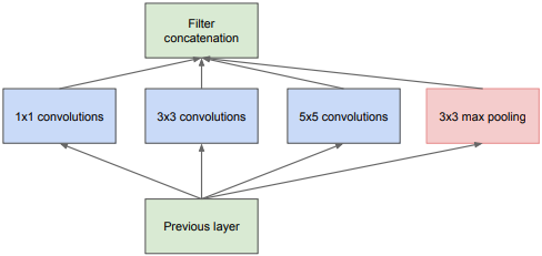
Thus, the structure shown in the figure below is generated. In this structure, 256 are evenly distributed in 3 × 3-scale features are transformed into multiple clusters with different scales, which can make the calculation more effective and converge faster. The following is the most original structure. Using the concatenation method mentioned in the previous section, different sizes of convolution kernels are used to obtain different sizes of features and fuse them. The sizes of convolution kernels 1, 3 and 5 are used to facilitate alignment: set the step size to 1, fill 0, 1 and 2 for the convolution kernels of three sizes respectively, and fill 1 for the pooling operation. The stacking of characteristic graphs of the same size can be realized through the concatenation method (the same size, channel addition).

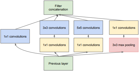
However, this structure is still not ideal, and the problem of calculation has not been well improved. For 5 × For the convolution kernel of 5, suppose for 100 × one hundred × 128 inputs use 256 5 × 5, the number of parameters will be up to (128 × five × 5+1) × 256=819456. If in use 5 × Before convolution, 32 1's are used × 1, the step size is 1, and the filling is 0, then 100 will be obtained × one hundred × 32, and 256 5 × If the convolution kernel of 5 is convoluted, the parameters of these two steps add up to only (128) × one × 1+1) × 32+(32 × five × 5+1) × 256 = 209184, the number of parameters is greatly reduced. The whole process is shown in the figure below. Inception v1 is obtained based on the above description.

Finally, summarize the characteristics of Inception v1:

1. The convolution layer has a common function, which can reduce and increase the dimension of the channel direction. Whether to reduce or increase depends on the number of channels (convolution cores) of the convolution layer;
2. Due to 1 × 1 convolution has only one parameter, which is equivalent to making a scale of the original feature map, and this scale is learned through training, which will improve the recognition accuracy;
3. The depth and width of the network are increased;
4. 1 is used at the same time × 1，3 × 3，5 × 5, which increases the adaptability of the network to scale.

3. 1 × 1 convolution

1 is used in the concept module × 1. Maybe many people have the same doubts as me when they first see this thing. 3 × 3,5 × What the hell is this? Actually, 1 × The emergence of convolution solves many problems and plays a great role, so we analyze a wave separately here.

one × 1 convolution first appears in Network in Network(NIN) Generally speaking, the main functions of this paper are as follows:

1. Reduce and upgrade the number of channels
2. Increase the nonlinearity of the network
3. Realize cross channel interaction and information integration
4. Achieve the effect equivalent to the full connection layer

For action 1, dimensionality reduction is mainly to reduce parameters. The discussion in the previous section is the best example. GoogLeNet is using 1 × After the convolution dimensionality reduction of 1, a more compact network structure is obtained. Although there are 22 layers in total, the number of parameters is only one twelfth of that of 8-layer AlexNet (of course, a large part of the reason is that the full connection layer is removed). The dimensionality increase is mainly to expand the number of channels of the network with the least parameters, such as 256 3 × The convolution kernel parameters of 3 are obviously larger than 256 1 × The convolution kernel of 1 is much larger.

For action 2, it is also easy to understand, because there is usually a nonlinear activation function behind the convolution layer, so use 1 × 1 convolution can increase the nonlinear characteristics on the premise of keeping the scale of the feature map unchanged (i.e. without losing resolution and changing height and width).

For function 3, it is actually the transformation between channels. This function may be abstract. Use 1 × 1 convolution kernel, the operation of reducing dimension and upgrading dimension is actually the linear combination change of information between channels. Take a chestnut: in a 3 × three × Add a 1 after the convolution kernel of 64 × one × 28, so we get 3 × three × 28 convolution kernel, the original 64 channels can be understood as cross channel linear combination, which has become 28 channels, which is the information interaction between channels.

For function 4, the example of replacing the full connection layer with the volume layer in the VGGNet test phase in the previous blog should be understandable.

4. Overall design

The structure of GoogLeNet is very complete. The original paper uses a whole side to show the network structure. The following is a screenshot of my pdf.

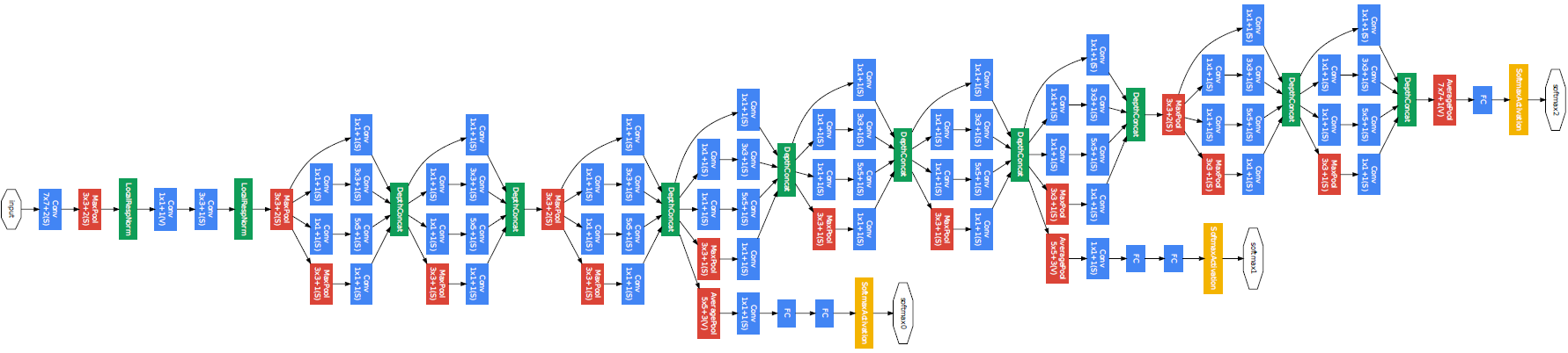
In fact, you can also look at the following table, which is also from the original paper. It is recommended that you go to the original paper Going deeper with convolutions
Look at the 4K large picture:

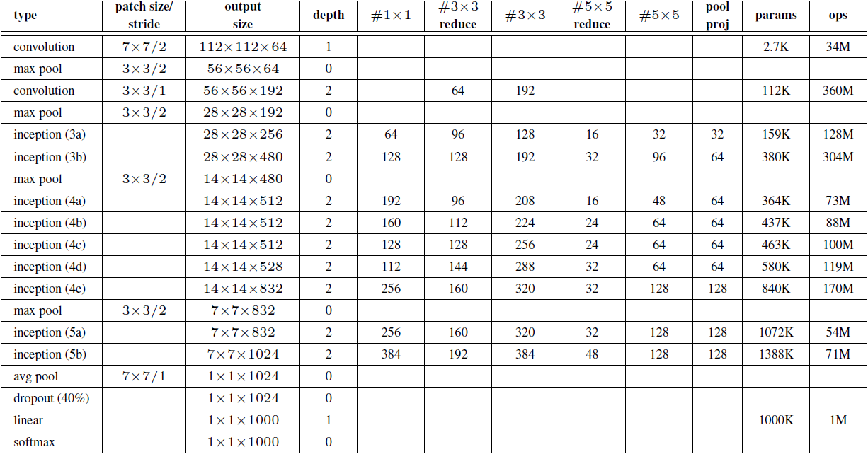
In #3 the above table × 3reduce,#5 × 5reduce means in 3 × 3,5 × 1 was used before the convolution operation of 5 × 1 convolution operation.

In addition to the previous discussion, the network has the following features:

1. Modular structure and combined splicing concept structure are adopted to facilitate adjustment;
2. Using the combination of average pooling and full connection layer, the experiment shows that this can improve the accuracy by 0.6%;
3. In order to avoid the problem of gradient disappearance, two additional auxiliary softmax functions are added to the network in order to enhance the speed of back propagation. During training, their losses will be weighted into the total loss of the network; They are not involved in classification during testing.

3, Example demonstration

First, implement the concept module. As can be seen from the previous figure, the Inception module has four parallel lines, and the first three lines use 1 respectively × 1,3 × 3 and 5 × The convolution kernel of 5 extracts the information under different spatial sizes, and the middle two lines will do 1 to the input × 1 convolution operation to reduce the number of input channels and reduce the complexity of the model. Line 4 will use 3 × 3. Maximize the pool layer, and then connect 1 × 1 convolution kernel changes the number of channels. Appropriate padding is used for all 4 lines, so that the height and width of the input and output characteristic diagrams are consistent. Finally, the output of each line is merged on the channel and input into the next layer. The implementation code of Inception v1 module is as follows:

import torch.nn as nn
import torch


def BasicConv2d(in_channels, out_channels, kernel_size):
    return nn.Sequential(
        nn.Conv2d(in_channels, out_channels, kernel_size, stride=1, padding=kernel_size // 2),
        nn.BatchNorm2d(out_channels),
        nn.ReLU(True)
    )


class InceptionV1Module(nn.Module):
    def __init__(self, in_channels, out_channels1, out_channels2reduce, out_channels2, out_channels3reduce,
                 out_channels3, out_channels4):
        super.__init__()
        # Line 1, single 1 × 1. Convolution
        self.branch1_conv = BasicConv2d(in_channels, out_channels1, kernel_size=1)
        # Line 2, 1 × 1 convolution followed by 3 × 3 convolution
        self.branch2_conv1 = BasicConv2d(in_channels, out_channels2reduce, kernel_size=1)
        self.branch2_conv2 = BasicConv2d(out_channels2reduce, out_channels2, kernel_size=3)
        # Line 3, 1 × 1 convolution followed by 5 × 5 convolution
        self.branch3_conv1 = BasicConv2d(in_channels, out_channels3reduce, kernel_size=1)
        self.branch3_conv2 = BasicConv2d(out_channels3reduce, out_channels3, kernel_size=5)
        # Line 4, 3 × 3 maximum pool layer followed by 1 × 1. Convolution
        self.branch4_pool = nn.MaxPool2d(kernel_size=3, stride=1, padding=1)
        self.branch4_conv = BasicConv2d(in_channels, out_channels4, kernel_size=1)

    def forward(self, x):
        out1 = self.branch1_conv(x)
        out2 = self.branch2_conv2(self.branch2_conv1(x))
        out3 = self.branch3_conv2(self.branch3_conv1(x))
        out4 = self.branch4_conv(self.branch4_pool(x))
        out = torch.cat([out1, out2, out3, out4], dim=1)
        return out

Assume that the original input image size is 224 × two hundred and twenty-four × 3. The first module of GoogLeNet uses a 64 channel convolution kernel with a size of 7 × The convolution layer of 7, stripe = 2, padding=3, and the output size is 112 × one hundred and twelve × 64. Perform ReLU operation after convolution. After 3 × After the maximum pool operation of 3 (stripe = 2), the output size is 56 × fifty-six × 64.

nn.Conv2d(3, 64, kernel_size=7, stride=2, padding=3),
nn.BatchNorm2d(64),
nn.ReLU(True),
nn.MaxPool2d(kernel_size=3, stride=2, padding=1)

The second module uses two convolution layers, first through 64 channel 1 × 1 roll up and then pass through 192 channels 3 × 3 convolution layer, corresponding to the second line from left to right in the Inception module.

nn.Conv2d(64, 64, kernel_size=1),
nn.Conv2d(64, 192, kernel_size=3, padding=1),
nn.BatchNorm2d(192),
nn.ReLU(True),
nn.MaxPool2d(kernel_size=3, stride=2, padding=1)

The third module Inception(3a): ① go through 1 first × one × 64, resulting in 28 × twenty-eight × 64 and sent to the ReLU activation function; ② Then go through 1 × one × 96, 28 × twenty-eight × 96 and sent to the ReLU activation function, and then passed through 3 × three × 128 (padding=1), and 28 is obtained × twenty-eight × Output characteristic diagram of 128; ③ After another 1 × one × 16, 28 × twenty-eight × 16 and sent to the ReLU activation function, and then passed through 5 × five × 32 (padding=2), and 28 is obtained × twenty-eight × 32 output characteristic diagram; ④ Finally, after 3 × The maximum pool operation of 3 (padding=1) is followed by 1 × one × 32, resulting in 28 × twenty-eight × Output characteristic diagram of 32. Combining the four branches into 64 + 128 + 32 + 32 = 256 channels, the size is 28 × twenty-eight × 256 output characteristic diagram. The calculation process of Inception(3b) and Inception(3a) is similar, and finally 480 channels are output.

InceptionV1Module(192, 64, 96, 128, 16, 32, 32),
InceptionV1Module(256, 128, 128, 192, 32, 96, 64),
nn.MaxPool2d(kernel_size=3, stride=2, padding=1)

The fourth module is a little more complicated, but it is very simple to understand, that is, five Inception modules are connected in series.

InceptionV1Module(480, 192, 96, 208, 16, 48, 64),
InceptionV1Module(512, 160, 112, 224, 24, 64, 64),
InceptionV1Module(512, 128, 128, 256, 24, 64, 64),
InceptionV1Module(512, 112, 144, 288, 32, 64, 64),
InceptionV1Module(528, 256, 160, 320, 32, 128, 128),
nn.MaxPool2d(kernel_size=3, stride=2, padding=1)

The fifth module is similar to the above module, but followed by the output layer. The module needs to use the average pooling layer to change the height and width of each channel to 1.

InceptionV1Module(832, 256, 160, 320, 32, 128, 128),
InceptionV1Module(832, 384, 192, 384, 48, 128, 128),
nn.AvgPool2d(kernel_size=7, stride=1)

Finally, after the output is turned into a two-dimensional array, a full connection layer with the number of output as the number of label categories is followed.

nn.Dropout(0.4),
nn.Linear(1024, num_classes)

The complete code is as follows:

class GoogLeNet(nn.Module):
    def __init__(self, num_classes):
        super().__init__()
        self.conv1 = nn.Sequential(
            nn.Conv2d(3, 64, kernel_size=7, stride=2, padding=3),
            nn.BatchNorm2d(64),
            nn.ReLU(True),
            nn.MaxPool2d(kernel_size=3, stride=2, padding=1)
        )
        self.conv2 = nn.Sequential(
            nn.Conv2d(64, 64, kernel_size=1),
            nn.Conv2d(64, 192, kernel_size=3, padding=1),
            nn.BatchNorm2d(192),
            nn.ReLU(True),
            nn.MaxPool2d(kernel_size=3, stride=2, padding=1)
        )
        self.inception3 = nn.Sequential(
            InceptionV1Module(192, 64, 96, 128, 16, 32, 32),
            InceptionV1Module(256, 128, 128, 192, 32, 96, 64),
            nn.MaxPool2d(kernel_size=3, stride=2, padding=1)
        )
        self.inception4 = nn.Sequential(
            InceptionV1Module(480, 192, 96, 208, 16, 48, 64),
            InceptionV1Module(512, 160, 112, 224, 24, 64, 64),
            InceptionV1Module(512, 128, 128, 256, 24, 64, 64),
            InceptionV1Module(512, 112, 144, 288, 32, 64, 64),
            InceptionV1Module(528, 256, 160, 320, 32, 128, 128),
            nn.MaxPool2d(kernel_size=3, stride=2, padding=1)
        )
        self.inception5 = nn.Sequential(
            InceptionV1Module(832, 256, 160, 320, 32, 128, 128),
            InceptionV1Module(832, 384, 192, 384, 48, 128, 128),
            nn.AvgPool2d(kernel_size=7, stride=1)
        )
        self.fc = nn.Sequential(
            nn.Dropout(0.4),
            nn.Linear(1024, num_classes)
        )

    def forward(self, x):
        x = self.conv1(x)
        x = self.conv2(x)
        x = self.inception3(x)
        x = self.inception4(x)
        x = self.inception5(x)
        x = x.view(x.size(0), -1)
        out = self.fc(x)
        return out

You can add the following FlattenLayer to the front of the full connection layer container to replace the x.view in forward, and use the following code to view the output size of each layer:

class FlattenLayer(nn.Module):
    def __init__(self):
        super().__init__()
        
    def forward(self, x):
        return x.view(x.size(0), -1)


net = GoogLeNet(1000)
X = torch.rand(1, 3, 224, 224)
for block in net.children():
    X = block(X)
    print('output shape: ', X.shape)

The output results are as follows:

output shape:  torch.Size([1, 64, 56, 56])
output shape:  torch.Size([1, 192, 28, 28])
output shape:  torch.Size([1, 480, 14, 14])
output shape:  torch.Size([1, 832, 7, 7])
output shape:  torch.Size([1, 1024, 1, 1])
output shape:  torch.Size([1, 1000])

4, Evolution improvement

The following is a brief introduction to the improvement of Inception v1: Inception v2. More variants such as Xception will not be discussed first. Later, there will be time to organize an inception series family. The reason why V2 is not introduced to the follow-up v3 is that many things in v3 have not been covered in the previous blog. The core idea of V2 is mentioned in VGGNet. Inception v2 and Inception v3 are in the same paper Rethinking the Inception Architecture for Computer Vision A paper on Batch Normalization is proposed Batch Normalization: Accelerating Deep Network Training by Reducing Internal Covariate Shift Not Inception v2. The difference between the two is that a variety of design and improvement technologies are mentioned in the paper. Some of the structures and improvement technologies are concept V2, and all of them are concept v3.

Based on concept V1, GoogLeNet team proposed two optimization methods: convolution kernel decomposition and feature graph size reduction. Because a larger convolution kernel size can bring a larger receptive field, but it will also bring more parameters and computation, GoogLeNet team proposed using two consecutive 3 × 3 convolution kernel instead of a 5 × 5 convolution kernel to reduce the number of parameters while maintaining the size of receptive field. First 3 × The convolution kernel of 3 obtains a 3 by convolution × 3, and then through a 3 × The convolution kernel of 3 produces a 1 × 1 characteristic diagram, output size and through a 5 × 5, and the number of parameters is reduced. A large number of experiments have proved that this substitution will not cause the loss of expression. This is also discussed in the last blog.

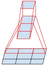
On this basis, the GoogLeNet team considered further decomposing the convolution kernel. For example, set 3 × The convolution kernel decomposition of 3 is shown in the figure below: first use 1 × The convolution kernel of 3 is convoluted, and then through 3 × The convolution kernel of 1 performs secondary convolution, and the final output size is the same as using a 3 × The convolution kernel of 3 has the same output size, and the number of parameters is reduced. So, an n × The convolution kernel of N can be represented by 1 × N and n × 1 is replaced by the combination of convolution kernels. The GoogLeNet team found that the effect of using this method in the lower layer of the network is not good, but it is better to use this method in the medium-sized feature map (it is recommended to use it in layers 12 to 20).

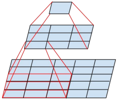
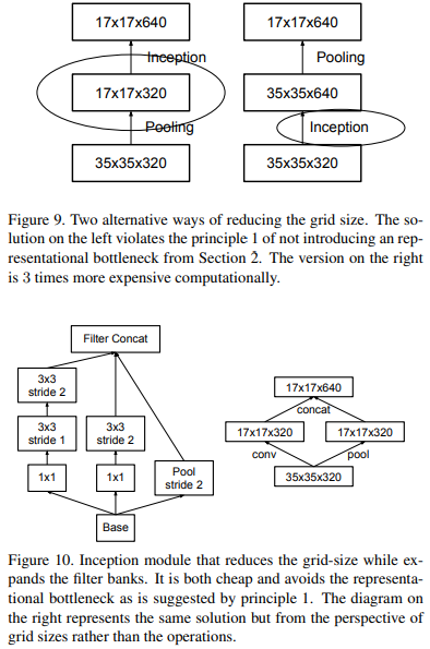
There are two ways to reduce the size of the feature map, as shown in the two structures above in the figure below: one is to perform pooling operation first, and then perform Inception convolution; Second, do the concept convolution first, and then perform the pooling operation. However, these two methods have disadvantages: using the method of pooling and then convolution is likely to lose some features; Using convolution first and then pooling, the amount of calculation will be very large. In order to reduce the amount of computation while maintaining the characteristics, the GoogLeNet team makes the convolution operation and pooling operation parallel, that is, separate calculation and then merge.

Unknowingly 1w many words orz, Batch Normalization can be recorded separately when there is time~