In the previous period, I learned how to summarize the results of univariate Cox regression. In this period, I learned the summary of univariate Logistic regression scores. Because the two functions of coxph * * * * and glm are used, the display of results is different, so the sorting process is slightly different, but the extracted information is consistent.

01 univariate Logistic regression analysis

Logistic regression model is a probability model. It takes the probability p of an event as the dependent variable and the factors affecting P as the independent variable to analyze the relationship between the probability of an event and the independent variable. It is a nonlinear regression model.

The Logistic regression model is applicable to the dependent variables:

1. binary taxonomy

2. Data of multiple classifications (ordered and disordered).

library(rms)#Realizable logistic regression model (lrm)
library(survival)
library("survminer")
data("lung")
head(lung)
table(lung$status)
  1   2 
 63 165 
 #Error in eval(family$initialize) : y values must be 0 <= y <= 1
lung$status=ifelse(lung$status==1,0,1)
table(lung$status)
 0   1 
 63 165 
fit<-glm(status~sex,family = binomial, data =lung)
summary(fit)
Call:
glm(formula = status ~ sex, family = binomial, data = lung)

Deviance Residuals: 
    Min       1Q   Median       3Q      Max  
-1.8271  -1.3333   0.6462   0.6462   1.0291  

Coefficients:
            Estimate Std. Error z value Pr(>|z|)    
(Intercept)   2.5614     0.4852   5.279  1.3e-07 ***
sex          -1.1010     0.3054  -3.605 0.000312 ***
---
Signif. codes:  0 '***' 0.001 '**' 0.01 '*' 0.05 '.' 0.1 ' ' 1

(Dispersion parameter for binomial family taken to be 1)

    Null deviance: 268.78  on 227  degrees of freedom
Residual deviance: 255.46  on 226  degrees of freedom
AIC: 259.46

Number of Fisher Scoring iterations: 4

Compare the results of glm with the results of coxph. The results of glm are not displayed after summary(). We need to calculate them separately. It has been introduced in the previous Logistic regression analysis. It is repeated here as follows:

fit<-glm(status~sex,family = binomial, data =lung)
sum<-summary(fit) ##Extract all regression results and put them into sum
OR<-round(exp(coef(fit)),2) ##1 - calculate the OR value and keep two decimal places
(Intercept)         sex 
      10.43        0.37
sum<-sum$coefficients[,2] ##Extract all regression results and put them into sum
Intercept)         sex 
  0.5513927   0.3529752 
SE<-sum$coefficients[,2] ##2-extract SE
(Intercept)         sex 
  0.5513927   0.3529752 
lower<-round(exp(coef(fit)-1.96*SE),2) # #3 - calculate CI, keep two decimal places and combine
(Intercept)         sex 
       3.54        0.19 
upper<-round(exp(coef(fit)+1.96*SE),2)
(Intercept)         sex 
      30.74        0.75 
P<-round(sum$coefficients[,4],2) # #4 - extract P value
(Intercept)         sex 
       0.00        0.01 

The following is the summary() of univariate Cox regression, which is obviously very different. Therefore, when sorting the results, we need to rewrite a simple function to obtain the results of batch regression.

02 batch single factor Logistic analysis

According to the above, calculate various indicators of each single factor Logistic regression analysis, such as OR, 95% confidence interval, P value, etc., sort them into a table, write a simple function, and obtain various indicators, as follows:

univ_formulas<- 
  function(x){
    #Fitting outcomes and variables
    fml<-as.formula(paste0("status==0~",x))
    #glm() logistic regression
    glm<-glm(fml,data=lung,family = binomial)
    #Extract all regression results and put them into sum
    sum<-summary(glm)
    #1 - calculate the OR value and keep two decimal places
    OR<-signif(exp(coef(glm)),2)
    #2-extract SE
    SE<-sum$coefficients[,2]
    #3 - calculate CI, keep two decimal places and combine
    lower<-signif(exp(coef(glm)-1.96*SE),2)
    upper<-signif(exp(coef(glm)+1.96*SE),2)
    CI<-paste0(lower,'-',upper)
    CI <- paste0(OR, " (", 
                  lower, "-", upper, ")")
    #4 - extract P value
    P<-signif(sum$coefficients[,4],2)
    #5 - merge the variable name, OR, CI and P into one table and delete the first row
    univ_formulas<- data.frame('Variants'=x,
                               'CI' = CI,
                               'P-value' = P,
                               'OR' = OR,
                               'lower' = lower,
                               'upper' = upper)[-1,]
                               
    #Return the loop function to continue the above operation                     
    return(univ_formulas)
  }

Here, we select 8 covariates other than time and status for univariate Logistic regression analysis, and then sort out the results to reach a table, which is the result of univariate Logistic regression analysis and a table that often appears in the article. Sort out the data as follows:

covariates <- c("inst","age", "sex",  "ph.karno", "ph.ecog", "wt.loss","meal.cal","pat.karno") 
univ_logistic_result <- lapply(covariates, univ_formulas)
univ_logistic_result
library(plyr)
univ_logistic_result <- ldply(univ_logistic_result,data.frame)
#Finally, change the value of P = 0 to P < 0.0001
univ_logistic_result$P.value[univ_logistic_result$P==0]<-"<0.001" 
names(univ_logistic_result)=c("Variants","Hazard Ratio (95%CI)","P-value","","","")
univ_logistic_result  #########The column names of the last three columns are assigned null values
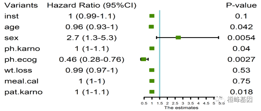
 Variants Hazard Ratio (95%CI) P-value               
1      inst         1 (0.99-1.1)     0.1 1.00 0.99 1.10
2       age        0.96 (0.93-1)   0.042 0.96 0.93 1.00
3       sex        2.7 (1.3-5.3)  0.0054 2.70 1.30 5.30
4  ph.karno            1 (1-1.1)    0.04 1.00 1.00 1.10
5   ph.ecog     0.46 (0.28-0.76)  0.0027 0.46 0.28 0.76
6   wt.loss        0.99 (0.97-1)    0.53 0.99 0.97 1.00
7  meal.cal              1 (1-1)    0.75 1.00 1.00 1.00
8 pat.karno            1 (1-1.1)   0.018 1.00 1.00 1.10
#Save as Excel
write.csv(univ_logistic_result ,"univ_logistic_result.csv",row.names = F)

03 univariate Logistic visualization

Here, we still use the R package forestplot to draw the visualization diagram, which is the same as that of single factor Cox regression, but the results are different. According to the above results, we have saved the output results. Next, we use read CSV () reads the result file as the input file, and the code of forest graph is the same as Cox regression, as follows:

#install.packages("forestplot")
library(forestplot)
rs_forest <- read.csv('univ_logistic_result.csv',header = FALSE)
rs_forest
# When reading data, you must set the header to FALSE to ensure that the first row is not called as a column name
 tiff('Figure 2.tiff',height = 1800,width = 3000,res= 600)
forestplot(labeltext = as.matrix(rs_forest[,c(1,2,3)]),
           #Set the columns for text display. Here, we use the first four columns of data as text and display them in the figure
           mean = rs_forest$V4, #Set average
           lower = rs_forest$V5, #Set the lowlimits of the mean value
           upper = rs_forest$V6, #Set the uplimits of the mean value
           #is.summary = c(T,T,T,T,T,T,T,T,T),
           #This parameter accepts a logical vector, which is used to define whether each row in the data is a summary value. If yes, it is set to TRUE at the corresponding position; if no, it is set to FALSE; Lines set to TRUE appear in bold
           zero = 1.5, #Set the reference value. Here we show the HR value, so the reference value is 1 instead of 0
           boxsize = 0.3, #Sets the estimated square size of the point
           lineheight = unit(8,'mm'),#Sets the line spacing in the drawing
           colgap = unit(2,'mm'),#Sets the spacing between columns in the drawing
           lwd.zero = 2,#Sets the thick green color of the guide line
           lwd.ci = 2,#Sets the thickness of the interval estimation line
           col=fpColors(box='#458B00', summary= "#8B008B",lines = 'black',zero = '#7AC5CD'),
           #Use the fpColors() function to define the color of graphic elements, and estimate the square, summary, interval estimation line and reference line from left to right
           xlab="The estimates",#Set x-axis power
           lwd.xaxis=2,#Sets the thick green color of the X axis
           lty.ci = "solid",
           graph.pos = 3)#Set the position of the forest map. If it is set to 4 here, it will appear in the fourth column
dev.off()

By comparing the results of single factor Cox regression analysis, we can see that the models used are different and the results obtained are quite different. I'm just taking an example here. Therefore, in model selection, we must clearly know what our purpose is, and the data type can accurately and quickly select the model.

When single factor is completed, single factor and multi factor need to be sorted into a table in the next period, and sometimes a column of grouping information of the data itself needs to be added, which will be explained in the next period.

Pay attention to the official account, update every day, remember to scan the code into groups, discuss every day, and exchange freely.

Reference:

1. Liu Y, Zhao P, Cheng M, Yu L, Cheng Z, Fan L, Chen C. AST to ALT ratio and arterial stiffness in non-fatty liver Japanese population:a secondary analysis based on a cross-sectional study. Lipids Health Dis. 2018 Dec 3;17(1):275.

2. Hosmer, D. & Lemeshow, S. (2000). Applied Logistic Regression (Second Edition). New York: John Wiley & Sons, Inc.

3. Long, J. Scott (1997). Regression Models for Categorical and Limited Dependent Variables. Thousand Oaks, CA: Sage Publications.

Huanfeng gene

Bioinformatics analysis, SCI article writing and bioinformatics basic knowledge learning: R language learning, perl basic programming, linux system commands, Python meet you better

31 original content

official account