
Gviz package introduction
Introduction to Gviz software package
The Gviz package aims to provide a structured visualization framework to draw any type of data along genomic coordinates. It also allows the integration of public genome annotation data from sources such as UCSC or ENSEMBL.
Like most genome browsers, individual types of genome features or data are represented by separate tracks.
By default, Gviz checks the validity of all provided chromosome names on UCSC (chromosomes must start with chr string).
You can decide to turn off this function by calling options(ucscChromosomeNames=FALSE)
In the following example, the UCSC Genome and chromosome 7 (chr7) on the mouse mm9 genome will be utilized
Drawing an AnnotationTrack diagram
Note that the AnnotationTrack constructor can accommodate many different types of input.
For example, the start and end coordinates of the annotation function can be used as a single parameter
start and end as data Frame or even as IRanges or GRangesList objects.
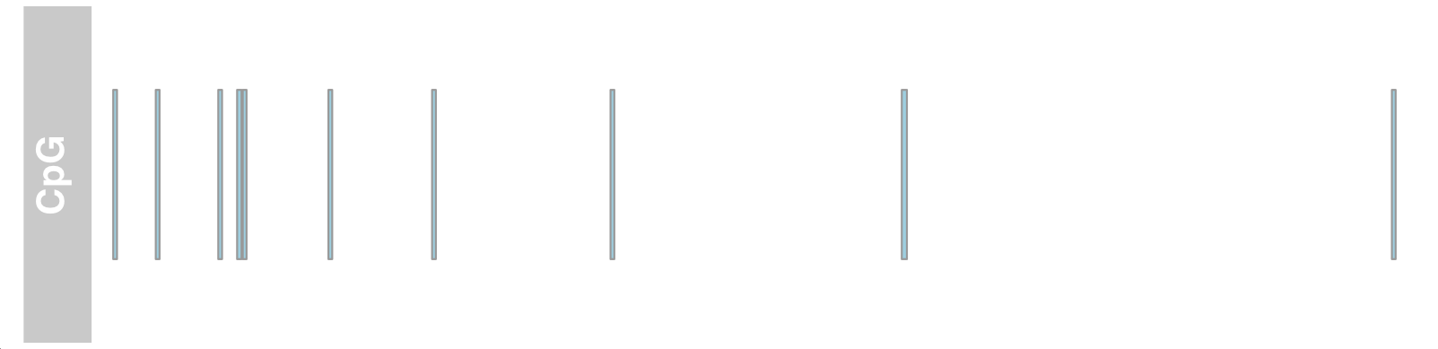
library(Gviz)
library(GenomicRanges)
#Load data: class = grades
data(cpgIslands)
cpgIslands

## GRanges object with 10 ranges and 0 metadata columns:
##        seqnames            ranges strand
##           <Rle>         <IRanges>  <Rle>
##    [1]     chr7 26549019-26550183      *
##    [2]     chr7 26564119-26564500      *
##    [3]     chr7 26585667-26586158      *
##    [4]     chr7 26591772-26593309      *
##    [5]     chr7 26594192-26594570      *
##    [6]     chr7 26623835-26624150      *
##    [7]     chr7 26659284-26660352      *
##    [8]     chr7 26721294-26721717      *
##    [9]     chr7 26821518-26823297      *
##   [10]     chr7 26991322-26991841      *
##   -------
##   seqinfo: 1 sequence from hg19 genome; no seqlengths
#Annotation track, titled "CpG"
atrack <- AnnotationTrack(cpgIslands, name = "CpG")
p<-plotTracks(atrack)
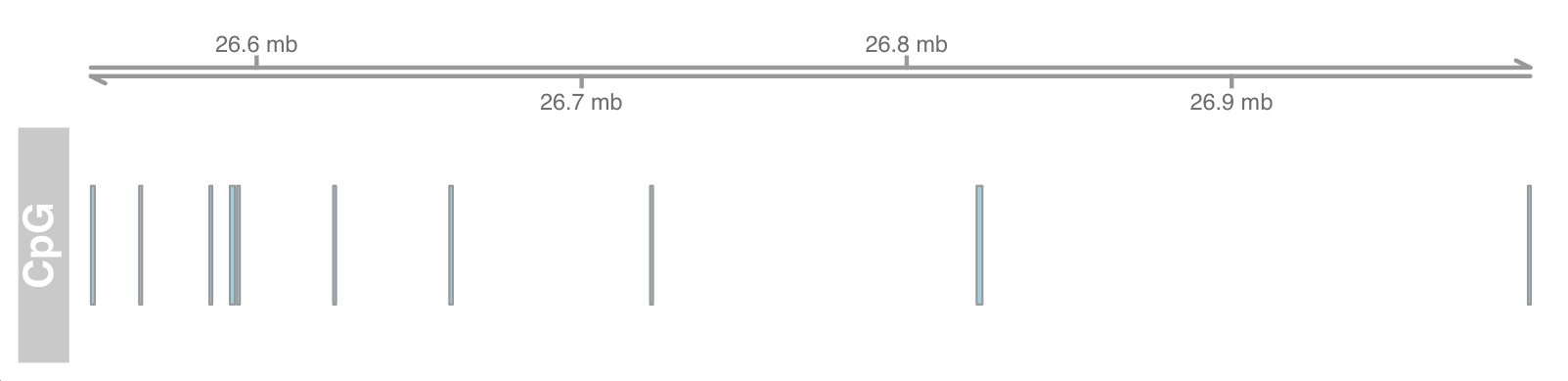
Add genome coordinates
## Genome coordinates
gtrack <- GenomeAxisTrack()
plotTracks(list(gtrack, atrack))
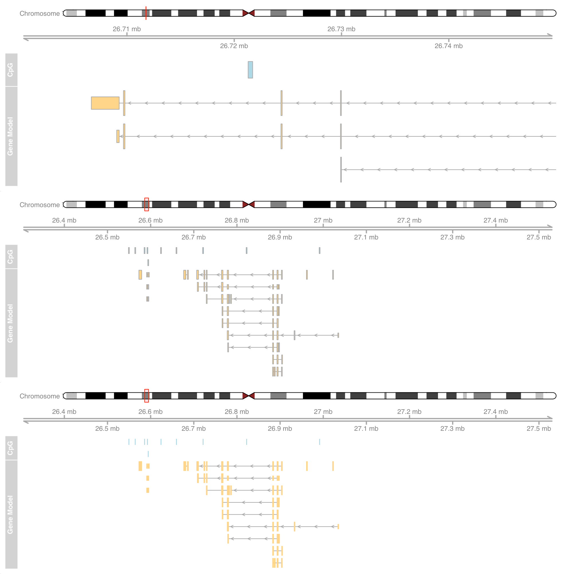
Add ideograph
To add a chromosome ideogram, we must specify a valid UCSC Genome (e.g. "hg19") and a chromosome name (e.g. "chr7")
Because this function obtains data from UCSC, an Internet connection is required, which may take a long time.
# genome : "hg19"
gen<-genome(cpgIslands)
# Chromosme name : "chr7"
chr <- as.character(unique(seqnames(cpgIslands)))
# Ideogram track
itrack <- IdeogramTrack(genome = gen, chromosome = chr)
plotTracks(list(itrack, gtrack, atrack))

Ideogram tracks are an exception to all Gviz track objects because they are not really displayed in the same coordinate system as all other tracks.
Instead, the current genome position is represented by a red box on the chromosome (or, in this case, a red line if the width is too small to accommodate the box).
Add gene model
We can use existing gene model information from local sources. Alternatively, you can download such data from one of the available online resources, such as UCSC or ENSEBML, and have constructors to handle these tasks.
For this example, we will start from the stored data Frame loads gene model data.
# Load data
data(geneModels)
head(geneModels)
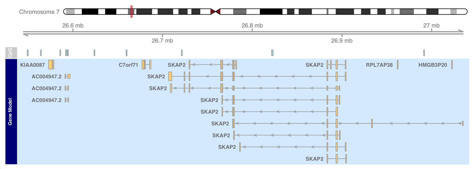
# Drawing
grtrack <- GeneRegionTrack(geneModels, genome = gen,
chromosome = chr, name = "Gene Model")
plotTracks(list(itrack, gtrack, atrack, grtrack))

Enlarge drawing
We often want to zoom in or out of a specific drawing area to see more details or a broader overview.
# Scale using the from and to parameters
plotTracks(list(itrack, gtrack, atrack, grtrack),
           from = 26700000, to = 26750000)

# Use extend Left and extend Right to zoom
# These parameters are relative to the current display range,
# And can be used to quickly expand the view at one or both ends of the drawing.
plotTracks(list(itrack, gtrack, atrack, grtrack),
           extend.left = 0.5, extend.right = 500000)

# Delete the boundary of exon to better show the picture
plotTracks(list(itrack, gtrack, atrack, grtrack),
           extend.left = 0.5, extend.right = 500000, col = NULL)
A value of 0.5 zooms in to half the current display range
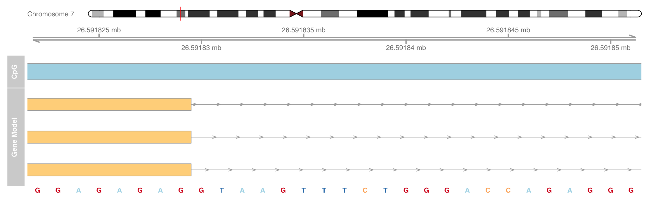
Add a sequence track and zoom in to see the sequence
The necessary sequence information comes from the BSgenome package
if (!requireNamespace("BiocManager", quietly = TRUE))
    install.packages("BiocManager")
BiocManager::install("BSgenome.Hsapiens.UCSC.hg19")

library(BSgenome.Hsapiens.UCSC.hg19)
strack <- SequenceTrack(Hsapiens, chromosome = chr)
plotTracks(list(itrack, gtrack, atrack, grtrack,
                strack), from = 26591822, to = 26591852, cex = 0.8)
Add data track
DataTrack objects are essentially run length coded (Rle) digital vectors or matrices that we can use to add various digital data to our genome coordinate map.
Different visualization options for these track s are available, including point diagram, histogram and box whisker diagram representation.
# For demonstration purposes, we can create a simple DataTrack object from randomly sampled data
set.seed(255)
lim <- c(26700000, 26750000)
coords <- sort(c(lim[1], sample(seq(from = lim[1],
                                    to = lim[2]), 99), lim[2]))
dat <- runif(100, min = -10, max = 10)
head(dat)
##data track
dtrack <- DataTrack(data = dat, start = coords[-length(coords)],
                    end = coords[-1], chromosome = chr, genome = gen,
                    name = "Uniform")

# Draw data track diagram
plotTracks(list(itrack, gtrack, atrack, grtrack,
                dtrack), from = lim[1], to = lim[2])

# Change the plot type to histogram
plotTracks(list(itrack, gtrack, atrack, grtrack,dtrack),
           from = lim[1], to = lim[2], type = "histogram")

This visualization is particularly useful when displaying, for example, the coverage of NGS reads along chromosomes, or displaying the measurements of mapping probes from microarray experiments.
Drawing parameters
Set parameters
#Annotation of transcript
# Change panel and title background color
grtrack <- GeneRegionTrack(geneModels, genome = gen,
                           chromosome = chr, name = "Gene Model",
                           transcriptAnnotation = "symbol",
                           background.panel = "#dbeeff",
                           background.title = "darkblue")
plotTracks(list(itrack, gtrack, atrack, grtrack))
Drawing direction
By default, all tracks are drawn in the 5 '- > 3' direction. Sometimes it is useful to actually display data relative to the opposite chain.
plotTracks(list(itrack, gtrack, atrack, grtrack),
           reverseStrand = TRUE)
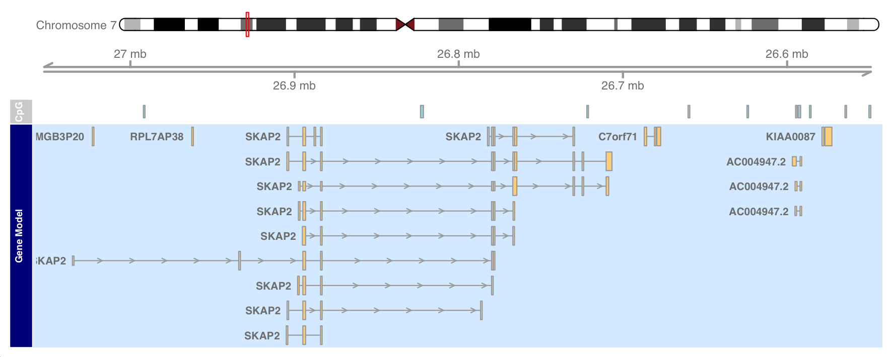
The data has been plotted on the reverse chain, which is also reflected in the GenomeAxis track.
Track classes
Several parameters can be used to change the appearance of different tracks.
Display parameters of GenomeAxisTrack
Set the position of the label to the bottom, display the ID, and change the color
axisTrack <- GenomeAxisTrack(range = IRanges(start = c(2000000,4000000), end = c(3000000, 7000000), names = rep("N-stretch", 2)))
plotTracks(axisTrack, from = 1000000, to = 9000000,
           labelPos = "below",showId=TRUE, col="#9400D3")

IdeogramTrack
#Ideogram
ideoTrack <- IdeogramTrack(genome = "hg19", chromosome = "chrX")
plotTracks(ideoTrack, from = 85000000, to = 129000000)

#Display chromosome band ID
plotTracks(ideoTrack, from = 85000000, to = 129000000,
           showId = FALSE, showBandId = TRUE, cex.bands = 0.4)

DataTrack
In essence, they constitute a run length encoded digital vector or matrix associated with a specific genomic coordinate range.
There can be multiple samples in a single dataset. The drawing method provides a tool for merging sample group information.
Therefore, the starting point for creating a DataTrack object will always be a set of ranges, in the form of IRanges or GRanges objects, or separately as start and end coordinates or widths. The second component is a numerical vector with the same length as the number of ranges, or a numerical matrix with the same number of columns.
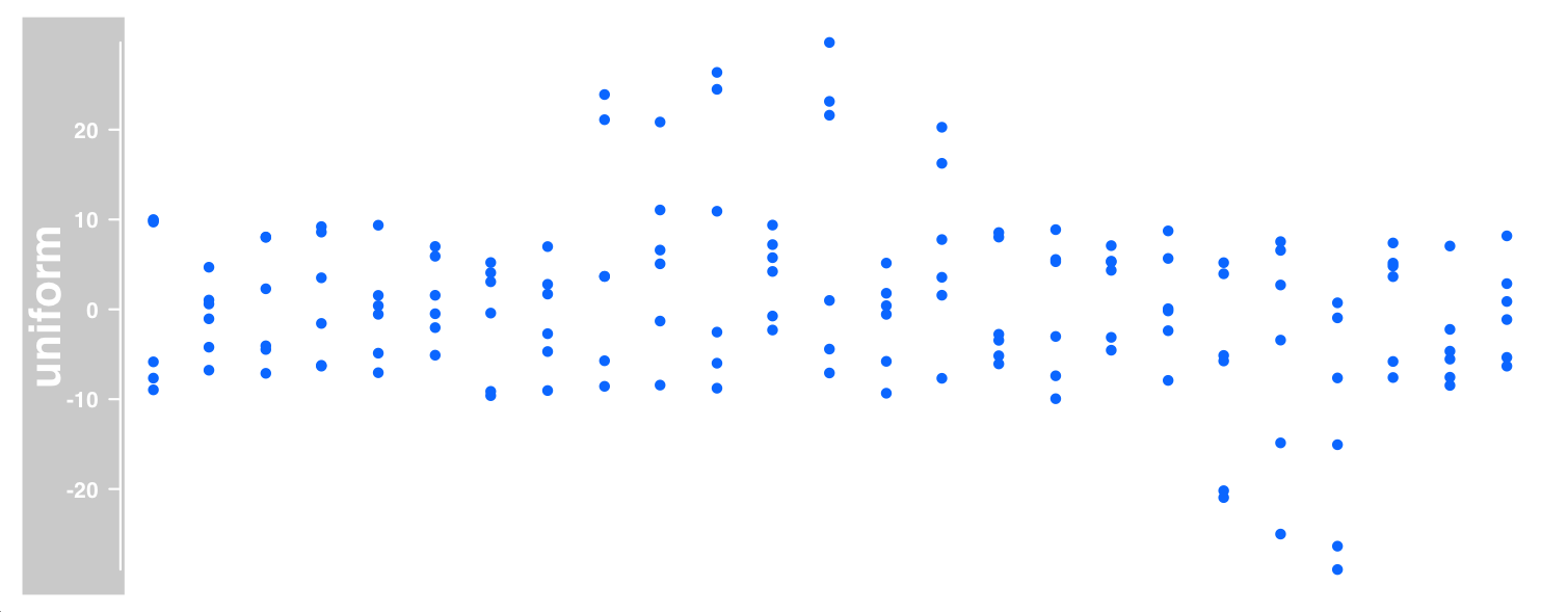
Next, we will load our sample data from the ranges object that is part of the Gviz package
# Load data
data(twoGroups)
head(twoGroups)
# data track diagram (the default visualization of DataTrack is point diagram)
 dTrack <- DataTrack(twoGroups, name = "uniform")
 plotTracks(dTrack)
Different picture types
Possible drawing types are:
# Point diagram
plotTracks(DataTrack(twoGroups, name = "p"), type="p")
# Line diagram
plotTracks(DataTrack(twoGroups, name = "l"), type="l")
# Line and point diagrams
plotTracks(DataTrack(twoGroups, name = "b"), type="b")
# Average chart
plotTracks(DataTrack(twoGroups, name = "a"), type="a")
# Straight line diagram
plotTracks(DataTrack(twoGroups, name = "h"), type="h")
# Histogram (bar width equals range)
plotTracks(DataTrack(twoGroups, name = "histogram"), type="histogram")
# 'polygon type' diagram
plotTracks(DataTrack(twoGroups, name = "polygon"), type="polygon")
# Box whisker diagram
plotTracks(DataTrack(twoGroups, name = "boxplot"), type="boxplot")
# Color image of each value
plotTracks(DataTrack(twoGroups, name = "heatmap"), type="heatmap")

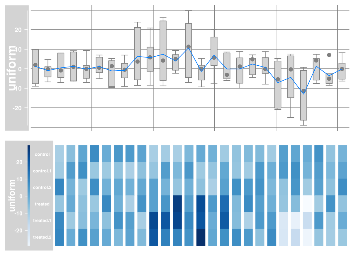
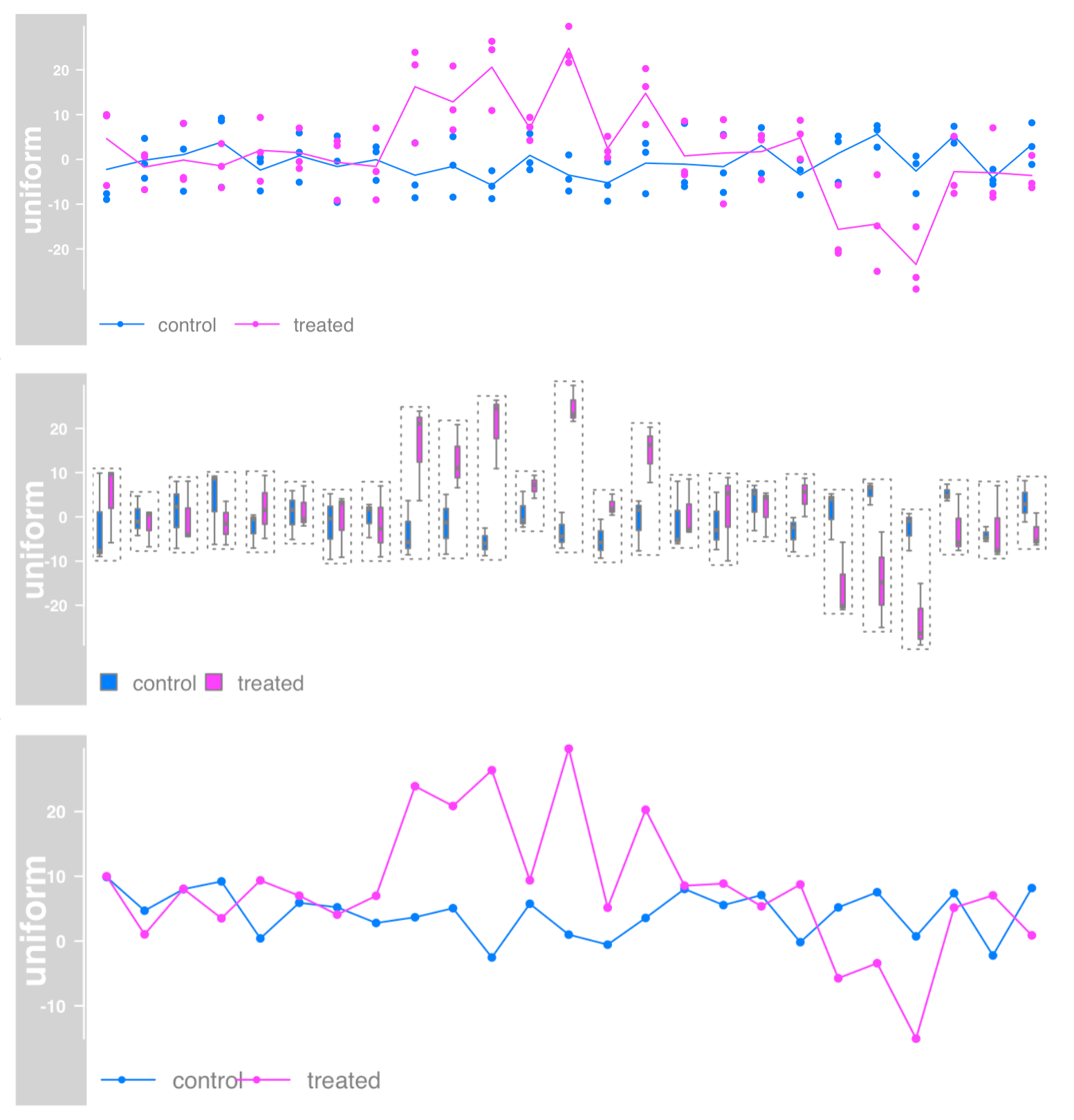
DataTrack diagram example:
# Combine boxplot with mean line and data grid (g):
plotTracks(dTrack, type = c("boxplot", "a", "g"))
# Heat map and display sample name
plotTracks(dTrack, type = c("heatmap"), showSampleNames = TRUE,
           cex.sampleNames = 0.6)
Data grouping
You can use factor variables to group individual samples together.
plotTracks(dTrack, groups = rep(c("control", "treated"), each = 3),
           type = c("a", "p"), legend=TRUE)
# Box diagram
plotTracks(dTrack, groups = rep(c("control", "treated"), each = 3),
           type = "boxplot")

# Aggregation group, which can be average, median, extreme, sum, minimum and maximum
plotTracks(dTrack, groups = rep(c("control", "treated"),each = 3),
           type = c("b"), aggregateGroups = TRUE,
           aggregation = "max")
Building DataTrack objects from files
The DataTrack class supports the most common file types, such as wig, bigWig, bedGraph, and bam files
bgFile <- system.file("extdata/test.bedGraph", package = "Gviz")
dTrack2 <- DataTrack(range = bgFile, genome = "hg19",
                     type = "l", chromosome = "chr19", name = "bedGraph")
plotTracks(dTrack2)
Note that the Gviz package uses the functionality in the rtracklayer package for most file import operations
Files in the Gviz package support streaming from index files.
Only relevant parts of the data need to be loaded during the drawing operation, so the underlying data file may be very large without reducing performance or causing too much memory consumption.
We will use the small bam file provided with the package here to illustrate this function.
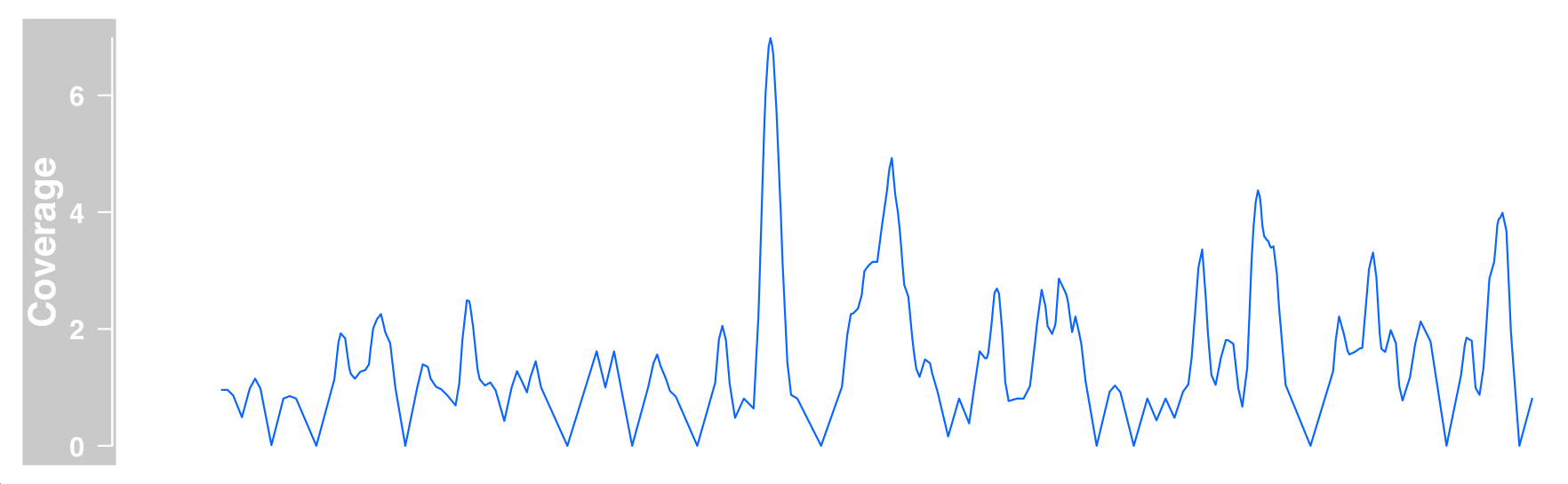
bam files contain alignment of sequences with common references. The most natural representation of such data in DataTrack is to view only the alignment coverage of a given location and encode it in a single elementMetadata column.
bamFile <- system.file("extdata/test.bam", package = "Gviz")
dTrack4 <- DataTrack(range = bamFile, genome = "hg19",
                     type = "l", name = "Coverage", window = -1, chromosome = "chr1")
plotTracks(dTrack4, from = 189990000, to = 190000000)
AnnotationTrack
Essentially, they consist of one or more genomic ranges that can be grouped into composite annotation elements if necessary.
The necessary building blocks are range coordinates, chromosomes, and genome identifiers.
Information can be passed to functions in the form of separate function parameters, such as IRanges, GRanges, or data Frame object.
aTrack <- AnnotationTrack(start = c(10, 40, 120),
                          width = 15, chromosome = "chrX", strand = c("+","*", "-"),
                          id = c("Huey", "Dewey", "Louie"),
                          genome = "hg19", name = "foo")
plotTracks(aTrack)

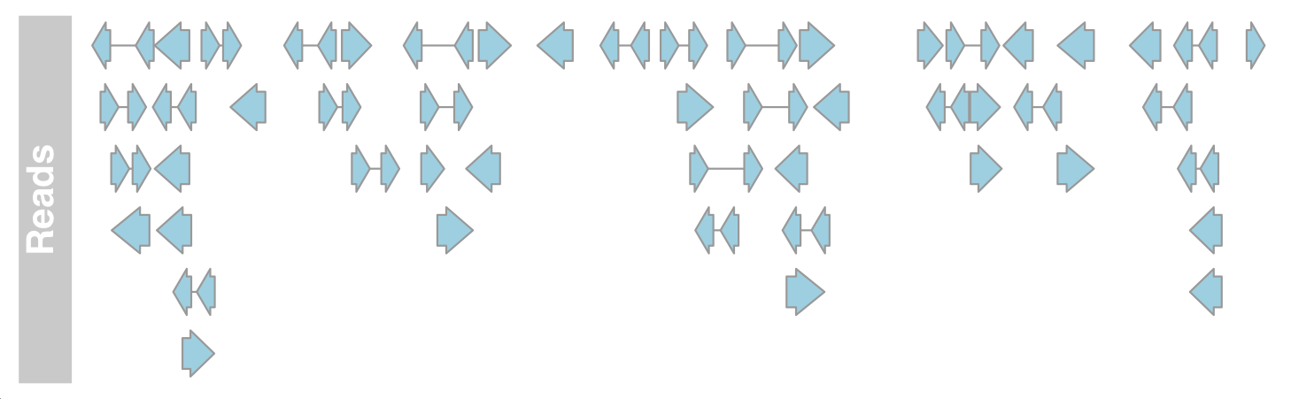
Building AnnotationTrack objects from files
The default import function reads the coordinates of all sequence alignments from the bam file.
#Annotation track
aTrack2 <- AnnotationTrack(range = bamFile, genome = "hg19",
                           name = "Reads", chromosome = "chr1")
plotTracks(aTrack2, from = 189995000, to = 190000000)
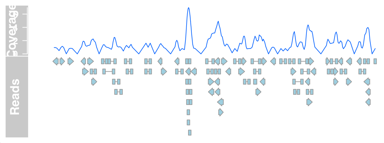
We can now draw DataTrack and AnnotationTrack representations of bam files at the same time to prove that the basic data is indeed the same.
plotTracks(list(dTrack4, aTrack2), from = 189990000,
           to = 190000000)
GeneRegionTrack
GeneRegionTrack is very similar to AnnotationTrack in principle.
The only difference is that they are more gene / transcript centric. We need to pass the start and end position (or width) of each annotation feature in the track, and provide exon, transcript and gene identifiers for each item, which will be used to create transcript groups.
A somewhat special case is to build GeneRegionTrack directly from one of the TranscriptDb. This option is described in more detail below.
data(geneModels)
grtrack <- GeneRegionTrack(geneModels, genome = gen,
                           chromosome = chr, name = "foo",
                           transcriptAnnotation = "symbol")
Building a GeneRegionTrack object from fTranscriptDbsx
The GenomicFeatures package provides a framework for downloading gene model information from online resources and storing it locally in the SQLite database.
One advantage of building GeneRegionTracks from TranscriptDb is that we get additional information about the coding and non coding regions of the transcript, that is, the coordinates of the 5 'and 3' UTR and CDS regions.
library(GenomicFeatures)
samplefile <- system.file("extdata", "UCSC_knownGene_sample.sqlite",
    package = "GenomicFeatures")
txdb <- loadDb(samplefile)
txTr <- GeneRegionTrack(txdb, chromosome = "chr6", start = 300000, end = 350000)
#feature(txTr)
plotTracks(txTr)
BiomartGeneRegionTrack
BiomartGeneRegionTrack, which provides a direct interface to ENSEMBL Biomart service.
We only need to input the genome, chromosome and the start and end positions on the chromosome. The constructor BiomartGeneRegionTrack will automatically contact ENSEMBL to obtain the necessary information and dynamically construct the gene model.
An Internet connection is required to work, and depending on usage and network traffic, contacting Biomart may take a lot of time.
biomTrack <- BiomartGeneRegionTrack(genome = "hg19",
                                    chromosome = chr, start = 20000000, end = 21000000,
                                    name = "ENSEMBL")
plotTracks(biomTrack, col.line = NULL, col = NULL)

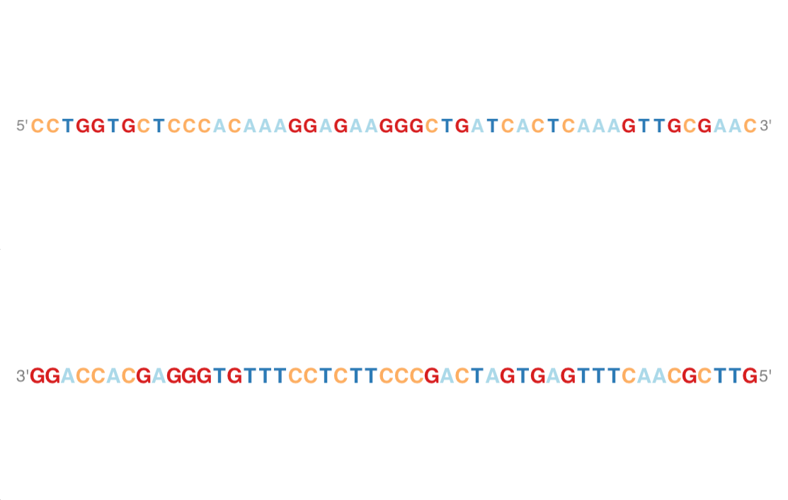
Sequence Track
library(BSgenome.Hsapiens.UCSC.hg19)
sTrack <- SequenceTrack(Hsapiens)
#sequence track : add 5'->3'
plotTracks(sTrack, chromosome = 1, from = 20000,to = 20050,
           add53=TRUE)
#The complement
plotTracks(sTrack, chromosome = 1, from = 20000,to = 20050,
           add53=TRUE, complement = TRUE)
AlignmentsTrack
The graph of aligned sequences, usually from next-generation sequencing experiments, may be very useful, such as when visually checking the effectiveness of what is called SNP. These comparisons are usually stored in BAM files.
RNA-seq
In this demonstration, let's use a small BAM file in which paired NGS reads have been mapped to extracts of the human hg19 genome.
The data are from RNA SEQ experiment. The comparison is carried out using STAR, and gaps are allowed.
Some gene annotation data of this region were also downloaded from Biomart.
afrom=2960000
ato=3160000
#bam file
alTrack <- AlignmentsTrack(system.file(package = "Gviz", "extdata", "gapped.bam"), isPaired = TRUE)
bmt <- BiomartGeneRegionTrack(genome = "hg19", chromosome = "chr12",
                              start = afrom, end = ato, filter = list(with_ox_refseq_mrna = TRUE),
                              stacking = "dense")
plotTracks(c(bmt, alTrack), from = afrom, to = ato, chromosome = "chr12")
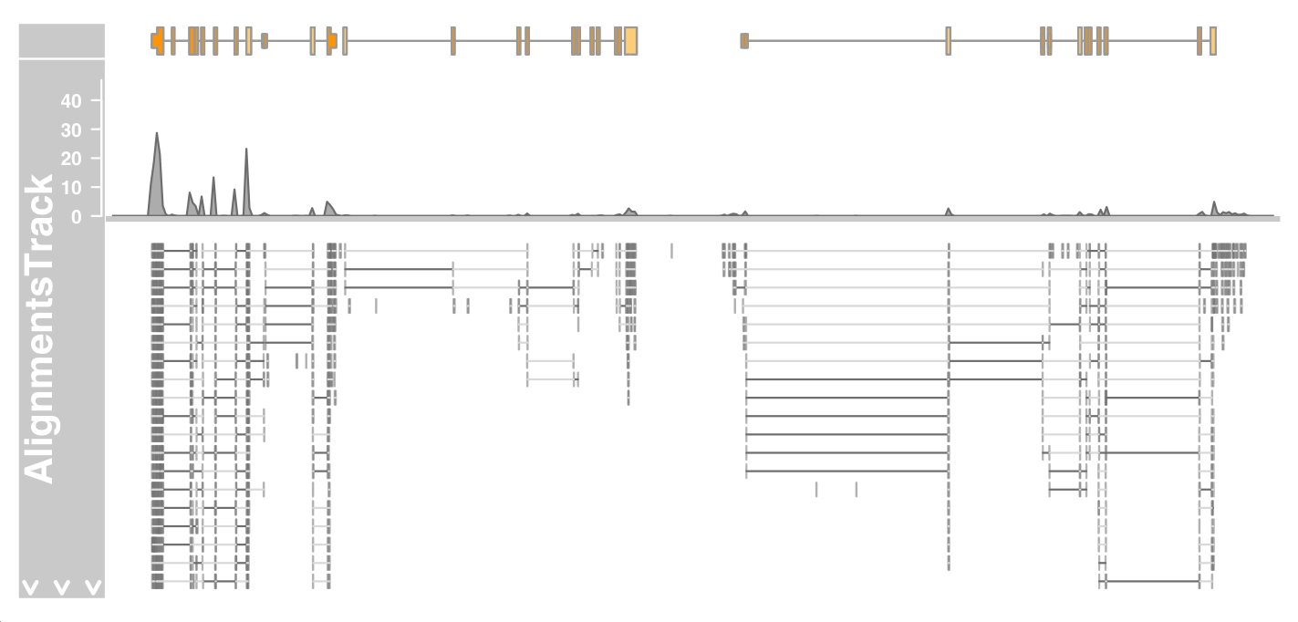
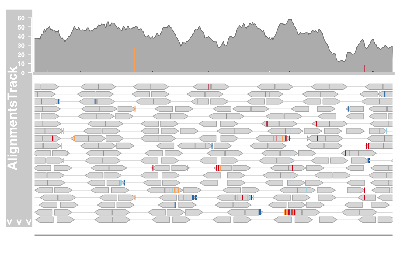
The figure above shows the overall layout of the track
At the top, we have a panel that displays the read coverage information in the form of a histogram. Below this panel, there is a stacked view of individual reads.
Only a certain space is available for drawing, and the whole stacking depth cannot be displayed here. The rest is indicated by the white down arrow in the title Panel.
We can solve this problem by using the max.height, min.height or stackHeight display parameters, which control the height or vertical spacing of stacked reads. Alternatively, we can reduce the size of the coverage area by setting the coverageHeight or minCoverageHeight parameters.
plotTracks(c(bmt, alTrack), from = afrom, to = ato,
           chromosome = "chr12", min.height = 0, coverageHeight = 0.08,
           minCoverageHeight = 0)

So far, pile ups are not particularly useful. We can turn them off by setting the type display parameters accordingly.
plotTracks(c(alTrack, bmt), from = afrom, to = ato, chromosome = "chr12", type = "coverage")

Zoom in further to see the details of the stacked part:
plotTracks(c(bmt, alTrack), from = afrom + 12700,
           to = afrom + 15200, chromosome = "chr12")
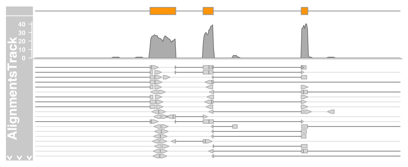
The direction of a single read is indicated by an arrow
read pairs are connected by bright gray lines
The gaps are displayed by a connected dark gray line
On devices that support transparency, we can also see that some reads actually overlap.
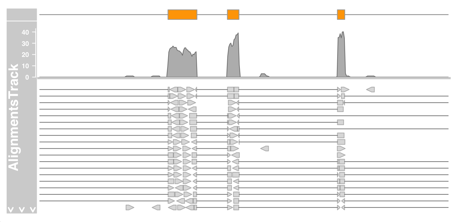
As mentioned earlier, we can control whether data should be treated as double ended data or single ended data by setting the isPaired parameter in the constructor.
Here is how we view the data in the same file in single ended mode
alTrack <- AlignmentsTrack(system.file(package = "Gviz",
                                       "extdata", "gapped.bam"), isPaired = FALSE)
plotTracks(c(bmt, alTrack), from = afrom + 12700,
           to = afrom + 15200, chromosome = "chr12")
DNA-seq
In order to better display the sequence variation characteristics of alignmenttrack, we will load different data sets, this time from genome-wide DNA SEQ SNP calling.
Similarly, the reference genome was hg19 and was compared using Bowtie2.
We need to specify alignmenttrack about the reference genome (sequenceTrack).
afrom <- 44945200
ato <- 44947200
alTrack <- AlignmentsTrack(system.file(package = "Gviz","extdata", "snps.bam"), isPaired = TRUE)
plotTracks(c(alTrack, sTrack), chromosome = "chr21", from = afrom,to = ato)
The mismatched bases are displayed in the form of superimposed histogram on the stacking part and a single read in the overlay.
When magnified to one of the obvious heterozygous SNP positions, more details can be revealed.
# enlarge
plotTracks(c(alTrack, sTrack), chromosome = "chr21", from = 44946590, to = 44946660)

# Show single letter
plotTracks(c(alTrack, sTrack), chromosome = "chr21",
           from = 44946590, to = 44946660, cex = 0.5, min.height = 8)

Track highlight and overlay
highlight
#highlight
ht <- HighlightTrack(trackList = list(atrack, grtrack,dtrack),
                     start = c(26705000, 26720000), width = 7000, chromosome = 7)
plotTracks(list(itrack, gtrack, ht), from = lim[1], to = lim[2])

superposition
For some applications, it makes sense to overlay multiple track s on the same area of the drawing.
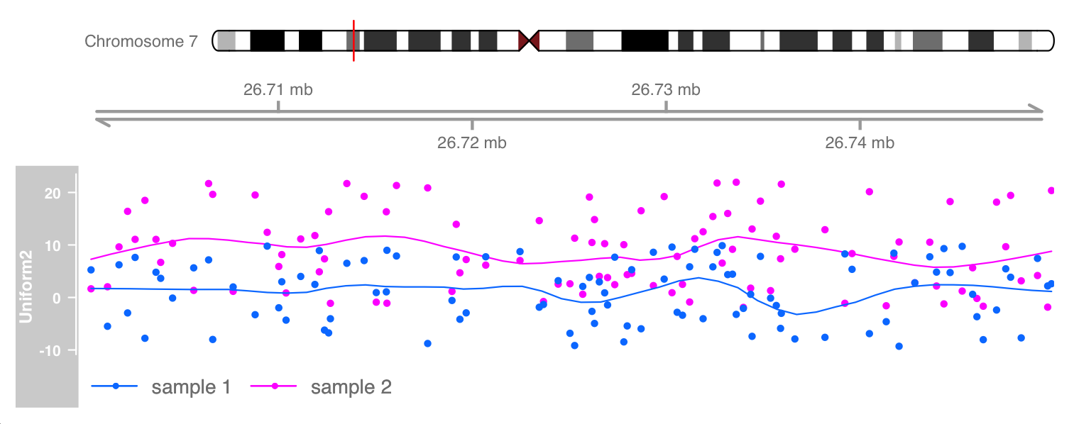
For example, we will generate a second DataTrack object and combine it with the existing objects in Chapter 2.
#create data
dat <- runif(100, min = -2, max = 22)
dtrack2 <- DataTrack(data = dat, start = coords[-length(coords)],
                     end = coords[-1], chromosome = chr, genome = gen,
                     name = "Uniform2", groups = factor("sample 2",levels = c("sample 1", "sample 2")),
                     legend = TRUE)
displayPars(dtrack) <- list(groups = factor("sample 1",levels = c("sample 1", "sample 2")), legend = TRUE)
ot <- OverlayTrack(trackList = list(dtrack2, dtrack))
ylims <- extendrange(range(c(values(dtrack), values(dtrack2))))
plotTracks(list(itrack, gtrack, ot), from = lim[1], to = lim[2], ylim = ylims, type = c("smooth", "p"))
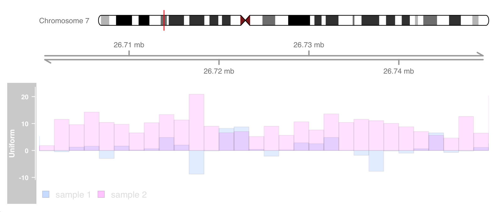
On devices that support it, alpha blending is a useful tool to sort out more information from track coverage, at least when comparing a small number of samples.
The resulting transparency effectively eliminates the problem of over drawing. The following example is only valid if this inset is built on a system with transparency blending support.
displayPars(dtrack) <- list(alpha.title = 1, alpha = 0.5)
displayPars(dtrack2) <- list(alpha.title = 1, alpha = 0.5)
ot <- OverlayTrack(trackList = list(dtrack, dtrack2))
plotTracks(list(itrack, gtrack, ot), from = lim[1],
           to = lim[2], ylim = ylims, type = c("hist"), window = 30)
reference resources
Gviz http://www.bioconductor.org/packages/release/bioc/html/Gviz.html
https://github.com/ivanek/Gviz
Hahne, Florian, and Robert Ivanek. 2016. "Statistical Genomics: Methods and Protocols." In, edited by Ewy Mathé and Sean Davis, 335–51. New York, NY: Springer New York. https://doi.org/10.1007/978-1-4939-3578-9_16.
Katz, Yarden, Eric T. Wang, Jacob Silterra, Schraga Schwartz, Bang Wong, Helga Thorvaldsdóttir, James T. Robinson, Jill P. Mesirov, Edoardo M. Airoldi, and Christopher B. Burge. 2015. "Quantitative Visualization of Alternative Exon Expression from Rna-Seq Data." Bioinformatics. https://doi.org/10.1093/bioinformatics/btv034.