[GiantPandaCV introduction] by introducing the variability ability of Deformable CNN on the basis of Transformer, we can reduce the amount of model parameters and improve the ability to obtain large receptive fields. Code interpretation is attached.

introduction

Transformer has stronger model representation ability because of its larger receptive field, and its performance exceeds many CNN models.

However, simply increasing the receptive field will also bring other problems. For example, the massive use of intensive attention in ViT will lead to the need for additional memory and computational cost, and the features are easily affected by irrelevant parts.

The spark attention used in PVT or swing transformer is unknown, which will affect the modeling ability of the model for long-distance dependence.

This introduces two features of the protagonist: deformable attention transformer:

• Data dependent: the position of key and value pairs depends on data.
• The combination of Deformable method can effectively reduce the computational cost and improve the computational efficiency.

The following figure shows motivation:

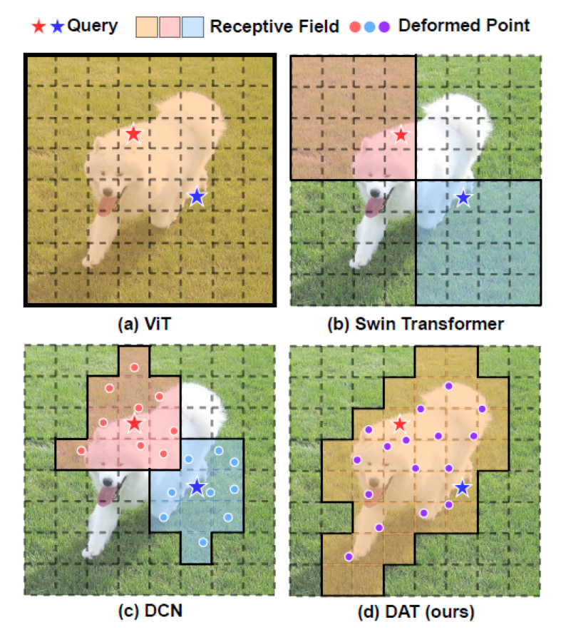
In the figure, the receptive fields of several methods are compared. Among them, red stars and blue stars represent different queries. The target wrapped by solid lines is the corresponding query processing area.

(a) ViT is the same for all queries. Because it uses global attention, the receptive field covers the whole picture.

(b) In swing transformer, attention based on window division is used. Different query processing locations are completed within a window.

(c) DCN uses 3x3 convolution kernel to add an offset, and the deviation is learned at 9 positions.

(d) DAT is the method proposed in this paper. Due to the combination of ViT and DCN, the response regions of all queries are the same, but these regions also learn the offset.

method

Recall the deformable Revolution:

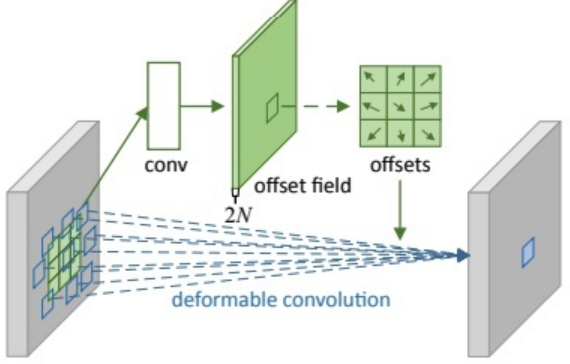
Simply put, an additional branch regression offset is used, and then it is loaded onto the coordinates to get the appropriate target.

Recall the multi head self attention in ViT:

With the above foreshadowing, the following figure is the core module of this article, Deformable Attention.

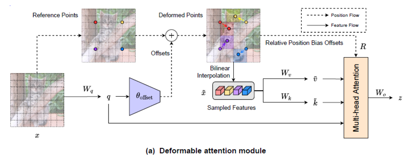
• The left part uses a set of reference points evenly distributed on the feature map
• Then, learn the offset value through the offset network and apply the offset to the reference point.
• After obtaining the reference point, use the bilinear pooling operation to extract a small part of the feature map as the input of k and v

x_sampled = F.grid_sample(
input=x.reshape(B * self.n_groups, self.n_group_channels, H, W), 
grid=pos[..., (1, 0)], # y, x -> x, y
mode='bilinear', align_corners=True) # B * g, Cg, Hg, Wg

• After that, the obtained Q, K and V execute ordinary self attention, and add relative position bias offsets on it.

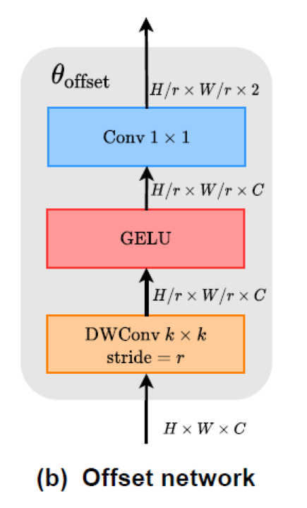
The construction of offset network is very simple. The code and diagram are as follows:

  self.conv_offset = nn.Sequential(
      nn.Conv2d(self.n_group_channels, self.n_group_channels, kk, stride, kk//2, groups=self.n_group_channels),
      LayerNormProxy(self.n_group_channels),
      nn.GELU(),
      nn.Conv2d(self.n_group_channels, 2, 1, 1, 0, bias=False)
  )

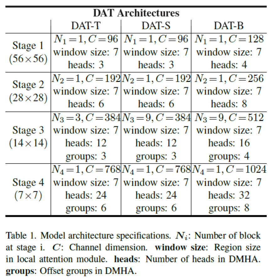
The final network structure is:

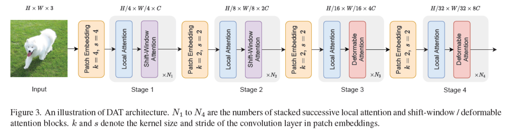
Specific parameters are as follows:

experiment

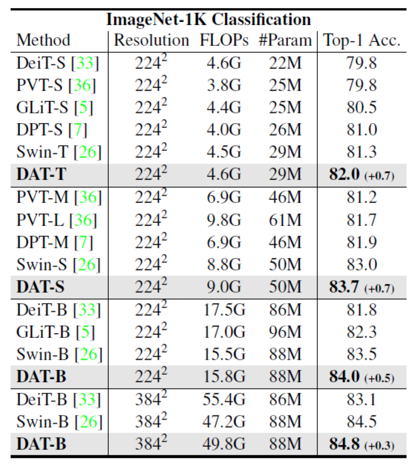
Experimental configuration: 300epoch, batch size 1024, lr=1e-3, data enhancement, most follow DEIT

• Classification results:

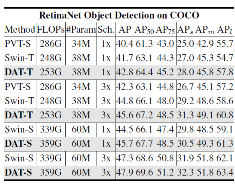
Target detection dataset results:

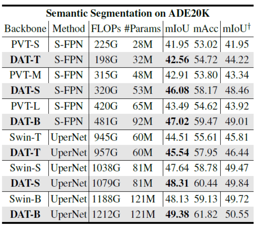
Semantic segmentation:

• Ablation Experiment:

• Visualization result: COCO

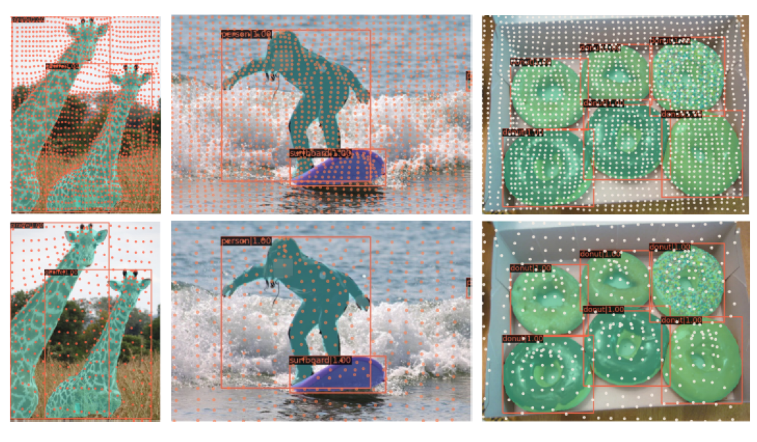
This visualization result is interesting. If most of the points distributed on the background do not change very much, that is, the offset is not very obvious, but there will be a certain concentration trend near the target (ps: this trend is not as obvious as the visualization result in Deformable Conv)

code

• Generate Q

  B, C, H, W = x.size()
  dtype, device = x.dtype, x.device
  
  q = self.proj_q(x)

• offset network is propagated forward to obtain offset

  q_off = einops.rearrange(q, 'b (g c) h w -> (b g) c h w', g=self.n_groups, c=self.n_group_channels)
  offset = self.conv_offset(q_off) # B * g 2 Hg Wg
  Hk, Wk = offset.size(2), offset.size(3)
  n_sample = Hk * Wk

• Use offset based on reference points

offset = einops.rearrange(offset, 'b p h w -> b h w p')
reference = self._get_ref_points(Hk, Wk, B, dtype, device)
    
if self.no_off:
    offset = offset.fill(0.0)
    
if self.offset_range_factor >= 0:
    pos = offset + reference
else:
    pos = (offset + reference).tanh()

• Use bilinear pooling to extract the corresponding feature map and wait for it to be input as K and V.

x_sampled = F.grid_sample(
    input=x.reshape(B * self.n_groups, self.n_group_channels, H, W), 
    grid=pos[..., (1, 0)], # y, x -> x, y
    mode='bilinear', align_corners=True) # B * g, Cg, Hg, Wg
    
x_sampled = x_sampled.reshape(B, C, 1, n_sample)

q = q.reshape(B * self.n_heads, self.n_head_channels, H * W)
k = self.proj_k(x_sampled).reshape(B * self.n_heads, self.n_head_channels, n_sample)
v = self.proj_v(x_sampled).reshape(B * self.n_heads, self.n_head_channels, n_sample)

• Introduce the offset of relative position in the positive encoding section:

  rpe_table = self.rpe_table
  rpe_bias = rpe_table[None, ...].expand(B, -1, -1, -1)
  
  q_grid = self._get_ref_points(H, W, B, dtype, device)
  
  displacement = (q_grid.reshape(B * self.n_groups, H * W, 2).unsqueeze(2) - pos.reshape(B * self.n_groups, n_sample, 2).unsqueeze(1)).mul(0.5)
  
  attn_bias = F.grid_sample(
      input=rpe_bias.reshape(B * self.n_groups, self.n_group_heads, 2 * H - 1, 2 * W - 1),
      grid=displacement[..., (1, 0)],
      mode='bilinear', align_corners=True
  ) # B * g, h_g, HW, Ns
  
  attn_bias = attn_bias.reshape(B * self.n_heads, H * W, n_sample)
  
  attn = attn + attn_bias

reference resources

https://github.com/LeapLabTHU/DAT

https://arxiv.org/pdf/2201.00520.pdf