OpenCV learning lesson from scratch - 6. Gray transformation and histogram processing

This series is for Python Xiaobai and explains the actual combat of OpenCV project from scratch.

The image processing method in spatial domain directly processes the pixels of the image. The image processing technology in spatial domain mainly includes gray transformation and spatial filtering.

This section introduces the gray level change and histogram processing of images, and provides complete routines and running results: binary processing, inverse color transformation, linear transformation, piecewise linear transformation, contrast stretching, gray level stratification, nonlinear transformation, histogram processing, histogram equalization, histogram matching, local histogram processing, statistics enhancement, back projection.

1. Image enhancement technology

Image Enhancement methods mainly include spatial domain transformation, frequency domain transformation and pseudo color processing.

• Spatial domain transformation: the spatial domain refers to the image plane. The image processing method in the spatial domain directly processes the pixels of the image. Spatial domain image processing technology mainly includes gray transformation and spatial filtering.
• Frequency domain transform: through Fourier transform, it is processed in the frequency domain, and then converted back to the spatial domain.
• Pseudo color processing: mapping gray image to color space, which is commonly used in remote sensing image and medical image processing.

2. Image graying and binarization

Images are classified according to color, which can be divided into binary image, gray image and color image.

• Binary image: an image with only black and white colors. Each pixel can be represented by 0 / 1, 0 for black and 1 for white.
• Grayscale image: only grayscale image. Each pixel is represented by an 8bit number [0255], such as 0 for pure black and 255 for pure white.
• Color image: color images are usually represented by a combination of three color channels: red (R), green (G) and blue (B).

BGR format is used for color images in OpenCV. The color image is grayed, which can be directly read as a grayscale image when reading the image file, or the color image can be converted into a grayscale image through the color space conversion function cv2.cvtColor.

Grayscale processing related functions and routines are described in [OpenCV learning lesson-2. Image reading and display].

# 1.1 image reading
    imgFile = "../images/imgLena.tif"  # Read the path of the file
    img1 = cv2.imread(imgFile, flags=1)  # flags=1 read color image (BGR)
    img2 = cv2.imread(imgFile, flags=0)  # flags=0 is read as a grayscale image

# 1.10 image display (plt.imshow)
    imgRGB = cv2.cvtColor(img1, cv2.COLOR_BGR2RGB)  # Image format conversion: BGR (openCV) - > RGB (pyqt5)
    imGray = cv2.cvtColor(img1, cv2.COLOR_BGR2GRAY)  # Image format conversion: BGR (openCV) - > gray    

Further, the image can be binarized by the function cv2.threshold.

Function Description:

cv2.threshold(src, thresh, maxval, type[, dst]) → retval, dst

The function threshold() can convert a gray image into a binary image. The image is completely composed of pixels 0 and 255, showing a visual effect of only black and white.

Gray thresholding through the selected gray threshold thresh, the gray value of each pixel is compared with the threshold, and the pixel with gray greater than the threshold is set as the maximum gray, and the pixel with gray less than the threshold is set as the minimum gray, so as to obtain a binary image, which can highlight the image contour and segment the target from the background.

Parameter Description:

• scr: input image of transformation operation, nparray two-dimensional array, which must be a single channel gray image!
• thresh: threshold, value range: 0 ~ 255
• maxval: fill color, value range 0 ~ 255, generally 255
• Type: transform type
  • cv2.THRESH_BINARY: set to 255 when it is greater than the threshold, otherwise set to 0
  • cv2.THRESH_BINARY_INV: set to 0 when it is greater than the threshold, otherwise set to 255
  • cv2.THRESH_TRUNC: set it to thresh when it is greater than the threshold, otherwise it will remain unchanged (keep the primary color)
  • cv2.THRESH_TOZERO: unchanged when it is greater than the threshold (keep the primary color), otherwise set to 0
  • cv2.THRESH_TOZERO_INV: set to 0 when it is greater than the threshold, otherwise it remains unchanged (keep the primary color)
  • cv2.THRESH_OTSU: use the OTSU algorithm to select the threshold
• Return value retval: returns the threshold value of binarization
• Return value dst: returns the output image of threshold transformation

be careful:

• 1. The function cv2.threshold binarizes the fixed threshold; The function cv2.adaptiveThreshold is a binarization processing function of adaptive threshold, which can dynamically adjust the threshold by comparing the relationship between pixels and surrounding pixels.
• 1. To be exact, only the type is cv2.THRESH_BINARY or cv2.THRESH_BINARY_INV is output as binary image, and threshold processing is performed for other transformation types, but it is not binary processing.

Routine: 1.47 binary transformation of image (fixed threshold)

    # 1.47 fixed threshold binary transformation
    img = cv2.imread("../images/imgLena.tif")  # Read color image (BGR)
    imgGray = cv2.imread("../images/imgLena.tif", flags=0)  # flags=0 is read as a grayscale image
    # imgGray = cv2.cvtColor(img, cv2.COLOR_BGR2GRAY)  # Color conversion: BGR (openCV) - > gray

    # cv2.threshold(src, thresh, maxval, type[, dst]) → retval, dst
    ret1, img1 = cv2.threshold(imgGray, 63, 255, cv2.THRESH_BINARY)  # Convert to binary image, thresh=63
    ret2, img2 = cv2.threshold(imgGray, 127, 255, cv2.THRESH_BINARY)  # Convert to binary image, thresh=127
    ret3, img3 = cv2.threshold(imgGray, 191, 255, cv2.THRESH_BINARY)  # Convert to binary image, thresh=191
    ret4, img4 = cv2.threshold(imgGray, 127, 255, cv2.THRESH_BINARY_INV)  # Inverse binary image, BINARY_INV
    ret5, img5 = cv2.threshold(imgGray, 127, 255, cv2.THRESH_TRUNC)  # TRUNC threshold processing, THRESH_TRUNC
    ret6, img6 = cv2.threshold(imgGray, 127, 255, cv2.THRESH_TOZERO)  # Tozero threshold processing, THRESH_TOZERO

    plt.figure(figsize=(9, 6))
    titleList = ["1. BINARY(thresh=63)", "2. BINARY(thresh=127)", "3. BINARY(thresh=191)", "4. THRESH_BINARY_INV", "5. THRESH_TRUNC", "6. THRESH_TOZERO"]
    imageList = [img1, img2, img3, img4, img5, img6]
    for i in range(6):
        plt.subplot(2, 3, i+1), plt.title(titleList[i]), plt.axis('off')
        plt.imshow(imageList[i], 'gray')  # Gray image ndim=2
    plt.show()

3. Gray scale transformation of image

Gray transformation is an important method of image enhancement, which can expand the dynamic range of the image, enhance the image contrast, make the image clearer and the features more obvious, so as to improve the display effect of the image.

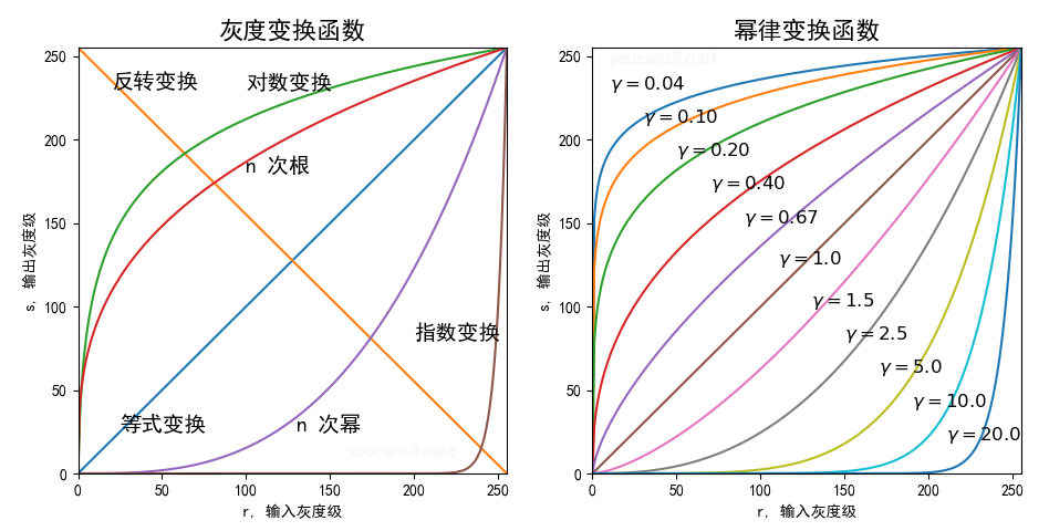
Gray transformation is to modify the gray value of each pixel of the image according to certain rules (gray mapping function), so as to change the dynamic range of image gray. According to the properties of gray-scale mapping function, gray-scale transformation can be divided into linear transformation, piecewise linear transformation and nonlinear transformation. Among the nonlinear transformation, logarithmic transformation, exponential transformation and power-law transformation (nth power and nth root) are the most commonly used. The shape of common gray transformation functions is shown in the figure below.

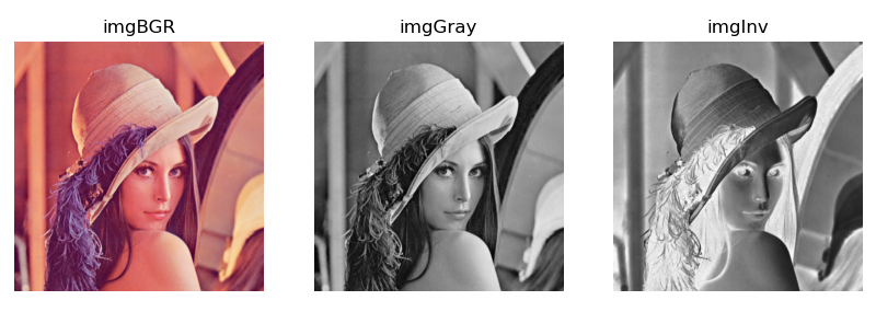
3.1 inverse color transformation (image inversion)

The inverse color transformation of the image, that is, image inversion, turns black pixels white and white pixels black. The generalized inverse color transformation can also be applied to color images, that is, all pixels are complemented.

The inversion processing of the image can enhance the white or gray details in the dark region.

Note the difference between image Invert and image Flip: image Flip is a geometric transformation along the axis of symmetry, and the pixel value remains unchanged; Image inversion is the reversal of pixel color, and the pixel position remains unchanged.

Routine: 1.48 inverse color transformation of image

    # 1.48 inverse color transformation of image
    img = cv2.imread("../images/imgLena.tif")  # Read color image (BGR)
    imgGray = cv2.cvtColor(img, cv2.COLOR_BGR2GRAY)  # Color conversion: BGR (openCV) - > gray
    h, w = img.shape[:2]  # The height and width of the picture

    # imgInv = np.zeros_like(img)  # Create a black image with the same shape as img
    imgInv = np.empty((w, h), np.uint8)  # Create a blank array
    for i in range(h):
        for j in range(w):
            imgInv[i][j] = 255 - imgGray[i][j]

    plt.figure(figsize=(10,6))
    plt.subplot(131), plt.imshow(cv2.cvtColor(img, cv2.COLOR_BGR2RGB)), plt.title("imgBGR"), plt.axis('off')
    plt.subplot(132), plt.imshow(imgGray, cmap='gray'), plt.title("imgGray"), plt.axis('off')
    plt.subplot(133), plt.imshow(imgInv, cmap='gray'), plt.title("imgInv"), plt.axis('off')
    plt.show()

3.2 linear grayscale transformation

Linear gray-scale transformation extends the dynamic range of the gray value of the original image to the specified range or the whole dynamic range according to the linear relationship.

The linear gray change makes a linear stretch on each pixel of the image, which can highlight the details of the image and improve the contrast of the image.

The linear grayscale transformation can be described by the following formula:
KaTeX parse error: No such environment: align at position 8: \begin{̲a̲l̲i̲g̲n̲}̲ Dt &= \frac{d-...
Where, D is the gray value of the original image, and Dt is the gray value of the image after linear gray transformation.

• When α = 1 ， β = 0 \alpha = 1，\beta = 0 α= 1， β= When 0, the original image remains unchanged
• When α = 1 ， β > 0 \alpha = 1，\beta > 0 α= 1， β> When 0, the gray value of the image moves up and the gray image color turns white (the color image color turns bright)
• When α = 1 ， β < 0 \alpha = 1，\beta < 0 α= 1， β< When 0, the gray value of the image moves down, and the gray image color is black (the color image color is dark)
• When α > 1 \alpha>1 α> 1, the contrast of the image is enhanced
• When 0 < α < 1 0 < \alpha < 1 0< α< 1, the contrast of the image decreases
• When α < 0 ， β = 255 \alpha < 0，\beta=255 α< 0 β= 255, the dark area of the image becomes bright, the bright area becomes dark, and the image is supplemented
• When α = − 1 ， β = 255 \alpha = -1，\beta = 255 α= −1， β= 255, the gray value of the image is reversed

Histogram normalization is a linear transformation that stretches the image to the whole gray level domain [0255] according to the minimum gray level and maximum gray level of the image.

Routine: 1.49 linear grayscale transformation of image

    # 1.49 linear gray scale transformation of image
    img = cv2.imread("../images/imgLena.tif")  # Read color image (BGR)
    imgGray = cv2.cvtColor(img, cv2.COLOR_BGR2GRAY)  # Color conversion: BGR (openCV) - > gray
    h, w = img.shape[:2]  # The height and width of the picture
    img1 = np.empty((w, h), np.uint8)  # Create a blank array
    img2 = np.empty((w, h), np.uint8)  # Create a blank array
    img3 = np.empty((w, h), np.uint8)  # Create a blank array
    img4 = np.empty((w, h), np.uint8)  # Create a blank array
    img5 = np.empty((w, h), np.uint8)  # Create a blank array
    img6 = np.empty((w, h), np.uint8)  # Create a blank array

    # Dt[i,j] = alfa*D[i,j] + beta
    alfa1, beta1 = 1, 50  # Alfa = 1, beta > 0: gray value moves up
    alfa2, beta2 = 1, -50  # Alfa = 1, beta < 0: gray value moves down
    alfa3, beta3 = 1.5, 0  # Alfa > 1, beta = 0: contrast enhancement
    alfa4, beta4 = 0.75, 0  # 0 < Alfa < 1, beta = 0: the contrast decreases
    alfa5, beta5 = -0.5, 0  # Alfa < 0, beta = 0: the dark area becomes bright and the bright area becomes dark
    alfa6, beta6 = -1, 255  # alfa=-1,beta=255: gray value inversion

    for i in range(h):
        for j in range(w):
            img1[i][j] = min(255, max((imgGray[i][j]+beta1), 0))  # Alfa = 1, beta > 0: white color
            img2[i][j] = min(255, max((imgGray[i][j]+beta2), 0))  # Alfa = 1, beta < 0: black color
            img3[i][j] = min(255, max(alfa3*imgGray[i][j], 0))  # Alfa > 1, beta = 0: contrast enhancement
            img4[i][j] = min(255, max(alfa4*imgGray[i][j], 0))  # 0 < Alfa < 1, beta = 0: the contrast decreases
            img5[i][j] = alfa5*imgGray[i][j]+beta5  # Alfa < 0, beta = 255: the dark area becomes bright and the bright area becomes dark
            img6[i][j] = min(255, max(alfa6*imgGray[i][j]+beta6, 0))  # alfa=-1,beta=255: gray value inversion

    plt.figure(figsize=(10, 6))
    titleList = ["1. imgGray", "2. beta=50", "3. beta=-50", "4. alfa=1.5", "5. alfa=0.75", "6. alfa=-0.5"]
    imageList = [imgGray, img1, img2, img3, img4, img5]
    for i in range(6):
        plt.subplot(2, 3, i + 1), plt.title(titleList[i]), plt.axis('off')
        plt.imshow(imageList[i], vmin=0, vmax=255, cmap='gray')
    plt.show()

3.3 piecewise linear gray scale transformation

Piecewise linear transformation function can enhance the contrast of each part of the image, enhance the gray range of interest and suppress the gray level of interest.

The advantage of piecewise linear function is that it can stretch the gray details of features according to needs. Some important transformations can only be described and realized by piecewise function. The disadvantage is that there are many parameters and it is not easy to determine.

The general formula of piecewise linear function is as follows:
D t = { c a D , 0 ≤ D < a d − c b − a [ D − a ] + c , a ≤ D ≤ b f − d e − b [ D − a ] + d , b < D ≤ e Dt = \begin{cases} \dfrac{c}{a} D &, 0 \leq D < a\\ \dfrac{d-c}{b-a}[D-a]+c &, a \leq D \leq b\\ \dfrac{f-d}{e-b}[D-a]+d &, b < D \leq e\\ \end{cases} Dt=⎩⎪⎪⎪⎪⎨⎪⎪⎪⎪⎧​ac​Db−ad−c​[D−a]+ce−bf−d​[D−a]+d​,0≤D<a,a≤D≤b,b<D≤e​
Where, D is the gray value of the original image, and Dt is the gray value of the image after linear gray transformation.

Routine: 1.50 piecewise linear grayscale transformation (contrast stretching)

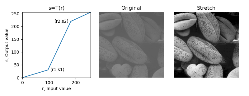
Contrast stretching can expand the gray level range in the image, so as to cover the ideal gray level range of the device.

The contrast stretching transformation function can have different implementation schemes, such as stretching the original gray range to a wide gray range; Or stretch the original gray range to the full domain gray range (0255); Or stretch the original gray range to a wide gray range, and truncate the lower or upper limit at the same time.

This routine makes (r1, s1) = (rMin, 0), (r2, s2) = (rmax, L-1), where rMin and rMax represent the minimum gray value and maximum gray value in the image, and linearly stretch the gray level of the original image to the whole range [0, L-1]. The left figure of the running result shows the stretching transformation curve of this routine.

    # 1.50 piecewise linear gray scale transformation (contrast stretching)
    imgGray = cv2.imread("../images/Fig0310b.tif", flags=0)  # flags=0 is read as a grayscale image
    height, width = imgGray.shape[:2]  # The height and width of the picture

    # constrast stretch, (r1,s1)=(rMin,0), (r2,s2)=(rMax,255)
    rMin = imgGray.min()  # The minimum value of the gray level of the original image
    rMax = imgGray.max()  # The maximum gray level of the original image
    r1, s1 = rMin, 0  # (x1,y1)
    r2, s2 = rMax, 255  # (x2,y2)

    imgStretch = np.empty((width, height), np.uint8)  # Create a blank array
    k1 = s1 / r1  # imgGray[h,w] < r1:
    k2 = (s2-s1) / (r2-r1)  # r1 <= imgGray[h,w] <= r2
    k3 = (255-s2) / (255-r2)  # imgGray[h,w] > r2
    for h in range(height):
        for w in range(width):
            if imgGray[h,w] < r1:
                imgStretch[h,w] = k1 * imgGray[h,w]
            elif r1 <= imgGray[h,w] <= r2:
                imgStretch[h,w] = k2 * (imgGray[h,w] - r1) + s1
            elif imgGray[h,w] > r2:
                imgStretch[h,w] = k3 * (imgGray[h,w] - r2) + s2

    plt.figure(figsize=(10,3.5))
    plt.subplots_adjust(left=0.2, bottom=0.2, right=0.9, top=0.8, wspace=0.1, hspace=0.1)
    plt.subplot(131), plt.title("s=T(r)")
    x = [0, 96, 182, 255]
    y = [0, 30, 220, 255]
    plt.plot(x, y)
    plt.axis([0,256,0,256])
    plt.text(105, 25, "(r1,s1)", fontsize=10)
    plt.text(120, 215, "(r2,s2)", fontsize=10)
    plt.xlabel("r, Input value")
    plt.ylabel("s, Output value")
    plt.subplot(132), plt.imshow(imgGray, cmap='gray', vmin=0, vmax=255), plt.title("Original"), plt.axis('off')
    plt.subplot(133), plt.imshow(imgStretch, cmap='gray', vmin=0, vmax=255), plt.title("Stretch"), plt.axis('off')
    plt.show()

Routine: 1.53 piecewise linear gray level transformation (gray level layering)

Gray level layering can highlight the specific gray level interval in the image, and the gray level can be processed by layering.

There are two common schemes for gray level layering: one is binary processing, which sets the gray level interval of interest as a larger gray value and the other as a smaller gray value; Another scheme is window processing, which sets the gray level interval of interest to a larger gray value, and the other intervals remain unchanged.

The segmented transformation formulas of the two gray level layering schemes are:
D t 1 = { d , a ≤ D ≤ b c , e l s e D t 2 = { d , a ≤ D ≤ b D , e l s e Dt_1 = \begin{cases} d &, a \leq D \leq b\\ c &, else \end{cases} \\ Dt_2 = \begin{cases} d &, a \leq D \leq b\\ D &, else \end{cases} Dt1​={dc​,a≤D≤b,else​Dt2​={dD​,a≤D≤b,else​
Where, D is the gray value of the original image, and Dt1 and Dt2 are the gray value of the image after gray transformation.

Routine 1.53 for the renal aortic angiography image, the gray level stratification technique is used to enhance the main blood vessels, and the gray level interval of interest is displayed in white. In scheme 1, binarization is performed, and other gray intervals are set to black; Scheme 2 keeps the gray values of other gray intervals unchanged.

    # # 1.53 Piecewise linear gray scale transformation (Gray level layering)  # Gray layered
    imgGray = cv2.imread("../images/Fig0312a.tif", flags=0)  # flags=0 is read as a grayscale image
    width, height = imgGray.shape[:2]  # The height and width of the picture

    # Gray layered strategy 1: binary image
    a, b = 155, 245  # Highlight the gray level of [a, b] interval
    imgLayer1 = imgGray.copy()
    imgLayer1[(imgLayer1[:,:]<a) | (imgLayer1[:,:]>b)] = 0  # Other areas: Black
    imgLayer1[(imgLayer1[:,:]>=a) & (imgLayer1[:,:]<=b)] = 255  # Grayscale window: white

    # Gray layered strategy 2: grayscale image
    imgLayer2 = imgGray.copy()
    imgLayer2[(imgLayer2[:,:]>=a) & (imgLayer2[:,:]<=b)] = 255  # Gray level window: white, other areas remain unchanged

    plt.figure(figsize=(10, 6))
    plt.subplot(131), plt.imshow(imgGray, cmap='gray'), plt.title('Original'), plt.axis('off')
    plt.subplot(132), plt.imshow(imgLayer1, cmap='gray'), plt.title('Binary layered'), plt.axis('off')
    plt.subplot(133), plt.imshow(imgLayer2, cmap='gray'), plt.title('Grayscale layered'), plt.axis('off')
    plt.show()

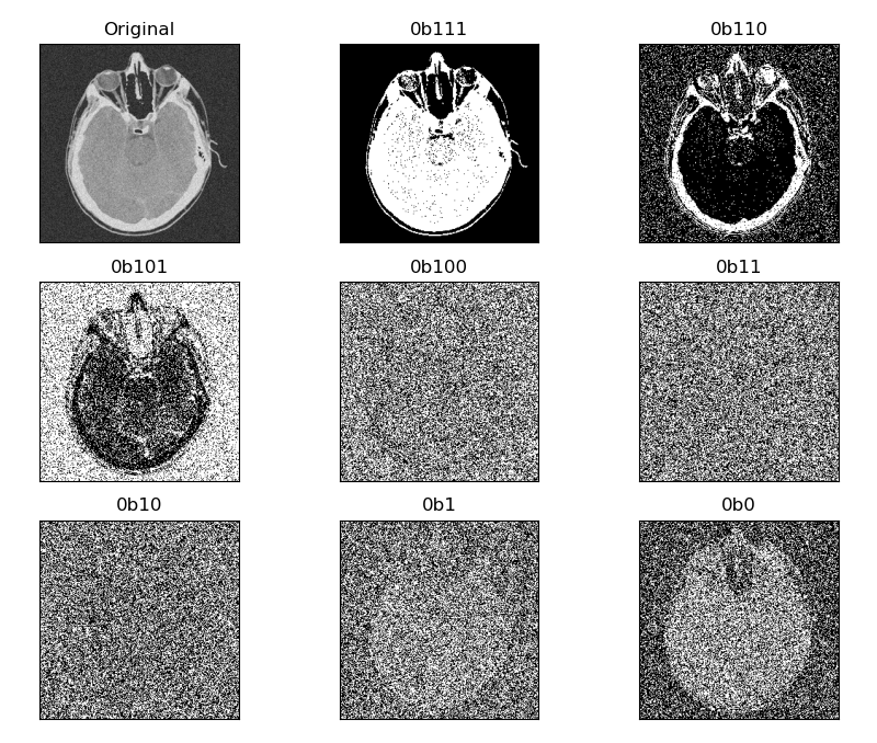
Routine: 1.54 piecewise linear grayscale transformation (bit plane layering)

The pixel value can also be expressed in binary form. By slicing each bit of the 8 bits binary number, 8 bit planes can be obtained, which is called bit plane slicing.
Generally, the high-order bit plane contains a large amount of visual data, while the low-order bit plane contains finer gray details. Therefore, bit plane layering can be used for image compression and image reconstruction.

    # # 1.54 piecewise linear grayscale transformation (bit plane slicing)
    img = cv2.imread("../images/Fig0726a.tif", flags=0)  # flags=0 is read as a grayscale image
    height, width = img.shape[:2]  # The height and width of the picture
    # imgRec = np.zeros((height, width), dtype=np.uint8)  # Create zero array

    plt.figure(figsize=(10, 8))
    for l in range(9, 0, -1):
        plt.subplot(3, 3, (9-l)+1, xticks=[], yticks=[])
        if l==9:
            plt.imshow(img, cmap='gray'), plt.title('Original')
        else:
            imgBit = np.empty((height, width), dtype=np.uint8)  # Create an empty array
            for w in range(width):
                for h in range(height):
                    x = np.binary_repr(img[w,h], width=8)  # Returns the binary representation of the input number as a string
                    x = x[::-1]
                    a = x[l-1]
                    imgBit[w,h] = int(a)  # Binary value of bit i
            plt.imshow(imgBit, cmap='gray')
            plt.title(f"{bin((l-1))}")
    plt.show()

3.4 nonlinear gray scale transformation: logarithmic transformation and exponential transformation

The logarithmic transformation can be described by the following formula:
D t = c ∗ l o g ( 1 + D ) Dt = c * log(1+D) Dt=c∗log(1+D)
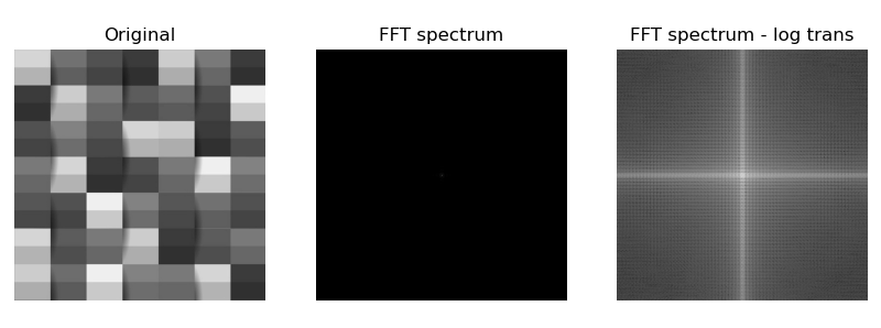
The slope of logarithmic curve is large in the area with low pixel value and small in the area with high pixel value. Logarithmic transformation maps the low gray value with narrow range in the input to the gray level with wide range, and the high gray value in the input is mapped to the gray level with narrow range. After logarithmic transformation, the contrast of darker areas is improved, which can enhance the dark details of the image.

The logarithmic transform realizes the effect of expanding the low gray value and compressing the high gray value, which is widely used in the display of spectrum images. The typical application of logarithmic transform is that the dynamic range of Fourier spectrum is very wide, and a large number of dark details are lost due to the limitation of the dynamic range of display equipment; After the dynamic range of the image is nonlinearly compressed by logarithmic transform, it can be clearly displayed.

Routine: 1.55 logarithmic transformation of image

    # 1.55 nonlinear gray scale transformation of image: logarithmic transformation
    img = cv2.imread("../images/Fig0305a.tif", flags=0)  # flags=0 is read as a grayscale image

    normImg = lambda x: 255. * (x-x.min()) / (x.max()-x.min()+1e-6)  # normalization
    fft = np.fft.fft2(img)  # Fourier transform
    fft_shift = np.fft.fftshift(fft)  # Centralization
    amp = np.abs(fft_shift)  # Fourier transform spectrum
    amp = np.uint8(normImg(amp))  # Map to [0, 255]
    ampLog = np.abs(np.log(1 + np.abs(fft_shift)))  # Logarithmic transformation
    ampLog = np.uint8(normImg(ampLog))  # Map to [0, 255]

    plt.figure(figsize=(9, 5))
    plt.subplot(131), plt.imshow(img, cmap='gray', vmin=0, vmax=255), plt.title('Original'), plt.axis('off')
    plt.subplot(132), plt.imshow(amp, cmap='gray', vmin=0, vmax=255), plt.title("FFT spectrum"), plt.axis('off')
    plt.subplot(133), plt.imshow(ampLog, cmap='gray', vmin=0, vmax=255), plt.title("FFT spectrum - log trans"), plt.axis('off')
    plt.tight_layout()
    plt.show()

3.5 nonlinear gray scale transformation: power law transformation (gamma transformation)

Power law transform, also known as gamma transform, can improve dark details and correct white (overexposed) or dark (underexposed) pictures.

The power-law transformation can be described by the following formula:
D t = c ∗ ( D + ϵ ) γ Dt = c * (D+\epsilon)^{\gamma} Dt=c∗(D+ϵ)γ
Gamma transform is essentially a power operation on each value in the image matrix$ 0 < \ gamma < 1 $, stretch the area with lower gray level in the image, compress the part with higher gray level, and increase the contrast of the image; γ > 1 \gamma >1 γ> 1, stretch the area with higher gray level in the image, compress the part with lower gray level, and reduce the contrast of the image.
Gamma transform compensates human visual characteristics through nonlinear transformation to maximize the use of effective gray level bandwidth. The brightness curves of many photographing, display and printing devices comply with power-law curves. Therefore, gamma transform is widely used in the adjustment of display effects of various devices, which is called gamma correction.

Routine: 1.56 power law transformation of image

    # 1.56 nonlinear gray scale transformation of image: power law transformation (gamma transform)
    img = cv2.imread("../images/imgB2.jpg", flags=0)  # flags=0 is read as a grayscale image

    gammaList = [0.125, 0.25, 0.5, 1.0, 2.0, 4.0]  # gamma value
    normImg = lambda x: 255. * (x-x.min()) / (x.max()-x.min()+1e-6)  # Normalized to [0255]

    plt.figure(figsize=(9,6))
    for k in range(len(gammaList)):
        imgGamma = np.power(img, gammaList[k])
        imgGamma = np.uint8(normImg(imgGamma))

        plt.subplot(2, 3, k+1), plt.axis('off')
        plt.imshow(imgGamma,  cmap='gray', vmin=0, vmax=255)
        plt.title(f"$\gamma={gammaList[k]}$")
    plt.show()

4. Histogram processing of image

4.1 gray histogram

Image histogram is a statistical table reflecting the distribution of image pixels. The abscissa represents the value range of pixel values, and the ordinate represents the total number or percentage of pixels in the image of each pixel value. Gray histogram is a function of image gray level, which is used to describe the number of pixels of each gray level in the image matrix.

The gray histogram reflects the gray distribution law in the image, intuitively shows the proportion of each gray level in the image, and well reflects the brightness and contrast information of the image: the center of the gray distribution indicates that the brightness is normal, the left indicates that the brightness is dark, and the right indicates that the brightness is high; Narrow and steep indicates low contrast, and wide and gentle indicates high contrast.

The image quality can be judged according to the shape of histogram, and the image quality can be improved by adjusting the shape of histogram.

OpenCV provides the function cv2.calcHist to calculate the histogram, and the function np.bincount in Numpy can also achieve the same function.

Function Description:

cv2.calcHist(images, channels, mask, histSize, ranges[, hist[, accumulate ]]) → hist

The function cv2.calcHist can calculate one-dimensional histogram or two-dimensional histogram. The parameters images, channels, histsize and ranges of the function should also be marked with [] when calculating one-dimensional histogram.

Parameter Description:

• images: input image, represented by [] brackets
• Channels: channels calculated by histogram, represented by [] brackets
• Mask: mask image, generally set to None
• histSize: the number of square columns, usually 256
• ranges: value range of pixel value, generally [0256]
• Return value hist: returns the total number of pixels in the image for each pixel value. The shape is (histSize,1)

be careful:

• 1. Parameters images, channels, histsize and ranges should all be marked with [].
• 1. Mask is a mask image with the same size as images, and the area with mask 0 is not processed. Set to None when no mask is used.
     3. channels is set to calculate the histogram for the specified channel of color image, and it is set to 0 for gray image.
     4. The function np.bincount in numpy can also achieve the same function, but the shape of the return value of this function is (histSize,)

Routine: 1.57 gray histogram of image

    # 1.57 gray histogram of image
    img = cv2.imread("../images/imgLena.tif", flags=0)  # flags=0 is read as a grayscale image

    histCV = cv2.calcHist([img], [0], None, [256], [0, 256])  # OpenCV functioncv2.calchist
    histNP, bins = np.histogram(img.flatten(), 256)
    print(histCV.shape, histNP.shape)  # histCV: (256, 1), histNP: (256,)

    plt.figure(figsize=(10,3))
    plt.subplot(131), plt.imshow(img, cmap='gray', vmin=0, vmax=255), plt.title("Original"), plt.axis('off')
    plt.subplot(132,xticks=[], yticks=[]), plt.axis([0,255,0,np.max(histCV)])
    plt.bar(range(256), histCV[:,0]), plt.title("Gray Hist(cv2.calcHist)")
    plt.subplot(133,xticks=[], yticks=[]), plt.axis([0,255,0,np.max(histCV)])
    plt.bar(bins[:-1], histNP), plt.title("Gray Hist(np.histogram)")
    plt.show()

4.2 histogram equalization

Histogram equalization is a simple and effective image enhancement technology. The image quality can be judged according to the shape of histogram, and the image quality can be improved by adjusting the shape of histogram.

Histogram equalization is to adjust the gray distribution of the original image through function transformation to obtain a new image with reasonable histogram distribution, so as to adjust the image brightness and enhance the contrast of the image with small dynamic range.

Due to the human visual characteristics, the image with uniform histogram has better visual effect. The basic idea of histogram equalization is to broaden the gray level with large proportion in the image and compress the gray level with small proportion, so as to make the histogram distribution of the image more uniform and expand the dynamic range of gray value difference, so as to enhance the overall contrast of the image.

Therefore, histogram equalization is to stretch the image nonlinearly and redistribute the image pixel value. In essence, it is to transform the image linearly or nonlinearly according to the histogram.

For example, histogram equalization can adjust the histogram of the original image to a uniform distribution, increase the dynamic range of gray value difference between pixels, and enhance the overall contrast of the image.

The distribution of the original image r can be transformed into the uniform distribution of s through the cumulative distribution function (CDF), which is the integral of the probability density function (PDF).

if p r ( r ) p_r(r) pr (r) and $p_s(s) $represents the probability density function of the original image r and the new image s, then:
s = T ( r ) = ( L − 1 ) ∫ 0 r p r ( r ) d r s=T(r)= (L-1) \int _0 ^r p_r(r) dr s=T(r)=(L−1)∫0r​pr​(r)dr
Its discrete form is:
s k = T ( r k ) = ( L − 1 ) ∑ j = 0 k p r ( r j ) = ( L − 1 ) ∑ j = 0 k n j N s_k = T(r_k) = (L-1) \sum_{j=0}^k p_r(r_j) = (L-1) \sum_{j=0}^k \frac{n_j}{N} sk​=T(rk​)=(L−1)j=0∑k​pr​(rj​)=(L−1)j=0∑k​Nnj​​
Therefore, the gray level of each pixel after equalization can be obtained directly from the histogram of the original image s k s_k sk to obtain the conversion function for histogram equalization:

(1) Calculate the histogram of the original gray image;

(2) The cumulative distribution function CDF of the original image is calculated by histogram accumulation;

(3) Based on the cumulative distribution function CDF, a new gray value is obtained by interpolation.

OpenCV provides the function cv2. equalizeHist, which can realize histogram equalization.

Function Description:

cv2.qualizeHist(src[, dst]) → dst

Parameter Description:

• src: input image
• Return value dst: output image, histogram equalization

Routine: 1.58 histogram equalization

    # 1.58 histogram equalization
    img = cv2.imread("../images/Fig0310b.tif", flags=0)  # flags=0 is read as a grayscale image

    imgEqu = cv2.equalizeHist(img)  # Use cv2.qualizeHist to complete histogram equalization transformation

    # histogram equalization image
    # histImg, bins = np.histogram(img.flatten(), 256)  # Calculate the histogram of the original image
    # cdf = histImg.cumsum()  # Calculate cumulative distribution function CDF
    # cdf = cdf * 255 / cdf[-1]  # CDF normalization of cumulative function: [0,1] - [0255]
    # imgEqu = np.interp(img.flatten(), bins[:256], cdf)  # Linear interpolation to calculate the new gray value
    # imgEqu = imgEqu.reshape(img.shape)  # Change the flattened image array into a two-dimensional array again

    fig = plt.figure(figsize=(7,7))
    plt.subplot(221), plt.title("Original image (youcans)"), plt.axis('off')
    plt.imshow(img, cmap='gray', vmin=0, vmax=255)  # original image 
    plt.subplot(222),plt.title("Hist-equalized image"), plt.axis('off')
    plt.imshow(imgEqu, cmap='gray', vmin=0, vmax=255)  # Convert image
    histImg, bins = np.histogram(img.flatten(), 256)  # Calculate the histogram of the original image
    plt.subplot(223, yticks=[]), plt.bar(bins[:-1], histImg)  # Original image histogram
    plt.title("Histogram of original image"), plt.axis([0,255,0,np.max(histImg)])
    histEqu, bins = np.histogram(imgEqu.flatten(), 256)  # Calculate the histogram of the original image
    plt.subplot(224, yticks=[]), plt.bar(bins[:-1], histEqu)  # Convert image histogram
    plt.title("Histogram of equalized image"), plt.axis([0,255,0,np.max(histImg)])
    plt.show()

4.3 histogram matching

Histogram equalization directly equalizes the image globally to generate an image with uniform histogram, regardless of the specific situation of local image area. For local areas and specific defects of an image, it is sometimes necessary to generate an image with a special shape histogram.

Histogram matching, also known as histogram specification, refers to adjusting the histogram of an image to a specified shape. For example, the histogram of an image or an area is matched to another image to keep the hue of the two images consistent.

This requires an inverse transformation on the basis of histogram equalization to adjust the histogram of uniform shape to the specified shape.

The main steps of histogram matching are:

(1) By specifying the histogram of the image z p z ( z ) p_z(z) pz (z), calculate its histogram equalization transformation s k s_k sk​；

(2) Pass s k s_k sk calculates the histogram equalization transformation function of image z G G G， G ( z q ) = s k G(z_q)=s_k G(zq​)=sk​；

(3) Calculate transformation function G G Inverse transformation function of G G − 1 G^{-1} G−1， z q = G − 1 ( s k ) z_q=G^{-1}(s_k) zq​=G−1(sk​)；

(4) The input image r is histogram equalized to obtain the equalized image s, and then the inverse transform function is used G − 1 G^{-1} G − 1 maps it to p z ( z ) p_z(z) pz (z) to obtain the histogram matching image Z. The two transformations in this step can also be combined into one.

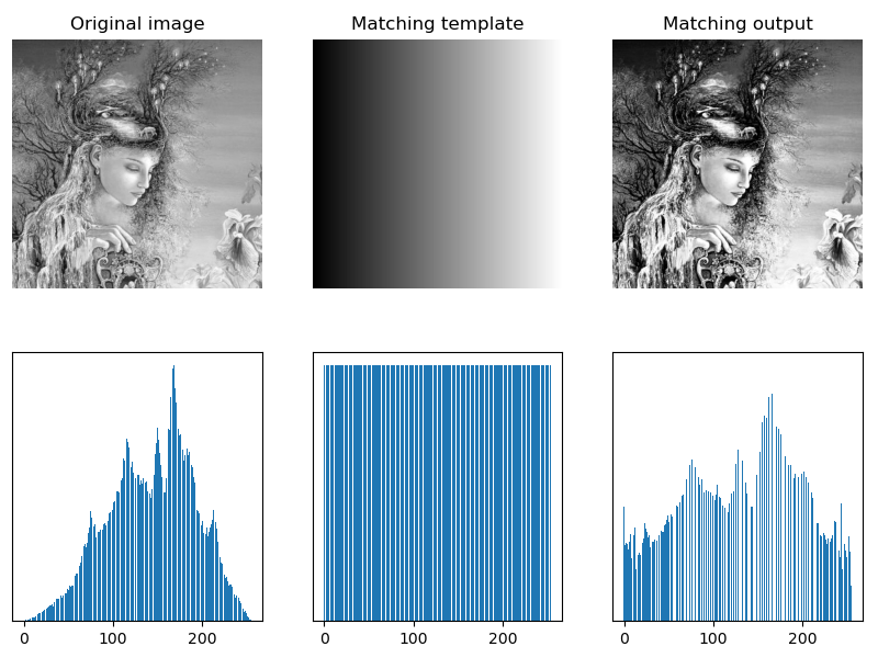
Routine: 1.59 gray image histogram matching

    # 1.59 gray image histogram matching
    img = cv2.imread("../images/imgGaia.tif", flags=0)  # flags=0 is read as a grayscale image
    imgRef = cv2.imread("../images/Fig0307a.tif", flags=0)  # matching template image

    # imgOut = calcHistMatch(img, imgRef)  # Subroutines: histogram matching

    # Calculate cumulative histogram
    histImg, bins = np.histogram(img.flatten(), 256)  # Calculate the histogram of the original image
    histRef, bins = np.histogram(imgRef.flatten(), 256)  # Calculate matching template histogram
    cdfImg = histImg.cumsum()  # Calculate the original image cumulative distribution function CDF
    cdfRef = histRef.cumsum()  # Calculate the matching template cumulative distribution function CDF

    # Calculate histogram matching conversion function
    transM = np.zeros(256)
    for i in range(256):
        index = 0
        vMin = np.fabs(cdfImg[i] - cdfRef[0])
        for j in range(256):
            diff = np.fabs(cdfImg[i] - cdfRef[j])
            if (diff < vMin):
                index = int(j)
                vMin = diff
        transM[i] = index

    # Histogram Matching 
    # imgOut = np.zeros_like(img)
    imgOut = transM[img].astype(np.uint8)

    fig = plt.figure(figsize=(10,7))
    plt.subplot(231), plt.title("Original image"), plt.axis('off')
    plt.imshow(img, cmap='gray')  # original image 
    plt.subplot(232), plt.title("Matching template"), plt.axis('off')
    plt.imshow(imgRef, cmap='gray')  # Matching template
    plt.subplot(233), plt.title("Matching output"), plt.axis('off')
    plt.imshow(imgOut, cmap='gray')  # Matching results
    histImg, bins = np.histogram(img.flatten(), 256)  # Calculate the histogram of the original image
    plt.subplot(234, yticks=[]), plt.bar(bins[:-1], histImg)
    histRef, bins = np.histogram(imgRef.flatten(), 256)  # Calculate matching template histogram
    plt.subplot(235, yticks=[]), plt.bar(bins[:-1], histRef)
    histOut, bins = np.histogram(imgOut.flatten(), 256)  # Calculate the histogram of matching results
    plt.subplot(236, yticks=[]), plt.bar(bins[:-1], histOut)
    plt.show()

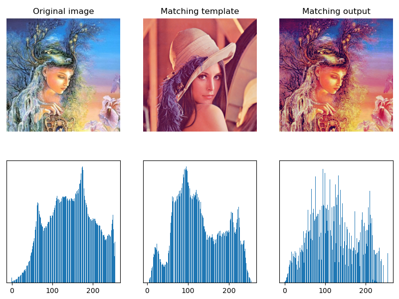
Routine: 1.60 color image histogram matching

    # 1.60 histogram matching of color image

    img = cv2.imread("../images/imgGaia.tif", flags=1)  # flags=1 is read as a color image
    imgRef = cv2.imread("../images/imgLena.tif", flags=1)  # Matching template image

    _, _, channel = img.shape
    imgOut = np.zeros_like(img)
    for i in range(channel):
        print(i)
        histImg, _ = np.histogram(img[:,:,i], 256)  # Calculate the histogram of the original image
        histRef, _ = np.histogram(imgRef[:,:,i], 256)  # Calculate matching template histogram
        cdfImg = np.cumsum(histImg)  # Calculate the original image cumulative distribution function CDF
        cdfRef = np.cumsum(histRef)  # Calculate the matching template cumulative distribution function CDF
        for j in range(256):
            tmp = abs(cdfImg[j] - cdfRef)
            tmp = tmp.tolist()
            index = tmp.index(min(tmp))  # find the smallest number in tmp, get the index of this number
            imgOut[:,:,i][img[:,:,i]==j] = index

    fig = plt.figure(figsize=(10,7))
    plt.subplot(231), plt.title("Original image"), plt.axis('off')
    plt.imshow(cv2.cvtColor(img, cv2.COLOR_BGR2RGB))  # Display original image
    plt.subplot(232), plt.title("Matching template"), plt.axis('off')
    plt.imshow(cv2.cvtColor(imgRef, cv2.COLOR_BGR2RGB))  # Show matching templates
    plt.subplot(233), plt.title("Matching output"), plt.axis('off')
    plt.imshow(cv2.cvtColor(imgOut, cv2.COLOR_BGR2RGB))  # Show matching results
    histImg, bins = np.histogram(img.flatten(), 256)  # Calculate the histogram of the original image
    plt.subplot(234, yticks=[]), plt.bar(bins[:-1], histImg)
    histRef, bins = np.histogram(imgRef.flatten(), 256)  # Calculate matching template histogram
    plt.subplot(235, yticks=[]), plt.bar(bins[:-1], histRef)
    histOut, bins = np.histogram(imgOut.flatten(), 256)  # Calculate the histogram of matching results
    plt.subplot(236, yticks=[]), plt.bar(bins[:-1], histOut)
    plt.show()

4.4 local histogram processing

Histogram equalization and histogram matching are based on the global transformation of the gray distribution of the whole image, not for the details of the local area of the image.

The idea of local histogram processing is to transform the histogram based on the gray distribution of the pixel neighborhood.

The process of local histogram processing is as follows:

(1) Set a template of a certain size (rectangular neighborhood) and move it pixel by pixel in the image;

(2) For each pixel position, calculate the histogram of the template area, perform histogram equalization or histogram matching transformation on the local area, and the transformation results are only used for the gray value correction of the central pixel of the template area;

(3) The template (neighborhood) moves row by row and column by column in the image, traverses all pixels, and completes the local histogram processing of the whole image.

OpenCV provides class cv2. createCLAHE to create adaptive equalization objects and methods, which can realize local histogram processing.

Function Description:

cv2.createCLAHE([, clipLimit[, tileGridSize]]) → retval

Parameter Description:

• clipLimit: threshold value of color contrast; optional; the default value is 8
• titleGridSize: template (neighborhood) size of local histogram equalization; optional; default value (8,8)

cv2. createCLAHE is a contrast limited adaptive histogram equalization method, which adopts the method of limiting histogram distribution and accelerated interpolation method.

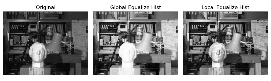
Basic routine: 1.61 adaptive local histogram equalization

    # 1.61 local histogram equalization
    img = cv2.imread("../images/FigClahe.jpg", flags=0)  # flags=0 is read as a grayscale image

    imgEqu = cv2.equalizeHist(img)  # Global histogram equalization
    clahe = cv2.createCLAHE(clipLimit=2.0, tileGridSize=(4,4))  # Create CLAHE object
    imgLocalEqu = clahe.apply(img)  # Adaptive local histogram equalization

    plt.figure(figsize=(9, 6))
    plt.subplot(131), plt.title('Original'), plt.axis('off')
    plt.imshow(img, cmap='gray', vmin=0, vmax=255)
    plt.subplot(132), plt.title(f'Global Equalize Hist'), plt.axis('off')
    plt.imshow(imgEqu, cmap='gray', vmin=0, vmax=255)
    plt.subplot(133), plt.title(f'Local Equalize Hist'), plt.axis('off')
    plt.imshow(imgLocalEqu, cmap='gray', vmin=0, vmax=255)
    plt.tight_layout()
    plt.show()

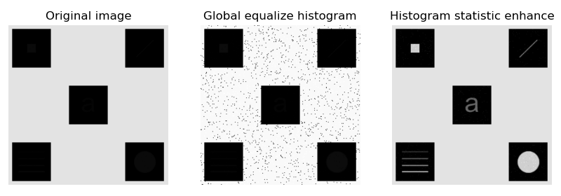
4.5 histogram statistics image enhancement

Histogram statistics image enhancement is to adjust the gray level and contrast of the image based on the histogram statistics information (such as mean and variance). Histogram statistics are not only used for global image enhancement, but also more effective in local image enhancement.

Local mean and variance are the basis of gray adjustment according to the characteristics of pixel neighborhood. The local mean of pixel neighborhood is the measure of average gray level, and the local variance is the measure of contrast. A simple and powerful image local enhancement algorithm can be developed by using local mean and variance.

The following is an introduction based on the methods and cases in Rafael C. Gonzalez's "Digital Image Processing (4th.Ed.).

The correction formula between the enhanced image g(x,y) and the original image f(x,y) is:
KaTeX parse error: No such environment: align at position 8: \begin{̲a̲l̲i̲g̲n̲}̲g(x,y)&=\begin{...

If the area to be enhanced is darker than the average gray level, you can choose k 0 = 0 , k 1 = 0.1 k_0 = 0, k_1 = 0.1 k0​=0,k1​=0.1； If the contrast of the area to be enhanced is very low, you can choose k 2 = 0 , k 3 = 0.1 k_2 = 0, k_3 = 0.1 k2​=0,k3​=0.1.

It should be pointed out that this method is only effective for some special types of images, and ROI setting and parameter adjustment need to be carried out for specific images in order to achieve better image enhancement effect.

Basic routine: 1.61 histogram statistics image enhancement

    # # 1.63 histogram statistics image enhancement
    img = cv2.imread("../images/Fig0326a.tif", flags=0)  # flags=0 is read as a grayscale image

    imgROI = img[12:120, 12:120]
    maxImg, maxROI = img.max(), imgROI.max()
    const = maxImg / maxROI
    imgHSE = enhanceHistStat(img, const)  # Subroutine: histogram statistics enhancement (custom method)

    plt.figure(figsize=(10, 6))
    plt.subplot(131), plt.title("Original image"), plt.axis('off')
    plt.imshow(img, cmap='gray', vmin=0, vmax=255)
    plt.subplot(132), plt.title("Global equalize histogram"), plt.axis('off')
    imgEqu = cv2.equalizeHist(img)  # Use cv2.qualizeHist to complete histogram equalization transformation
    plt.imshow(imgEqu, cmap='gray', vmin=0, vmax=255)
    plt.subplot(133), plt.title("Histogram statistic enhance"), plt.axis('off')
    plt.imshow(imgHSE, cmap='gray', vmin=0, vmax=255)
    plt.show()

4.6 histogram back projection (back tracking)

Histogram back projection is a method to find the best matching point or region with a specific template image in the input image. It can find and track specific color objects and specific gray objects. It is often used in image search and image segmentation.

The principle of histogram back projection processing is to calculate the histogram model of a feature, and then use the model to find the features in the image.

In the process of histogram back projection processing, first establish the histogram of the template area, then project the histogram to the input image, calculate the matching probability between the pixel value and the histogram of each pixel in the input image, obtain the probability image, and binarize it with a certain threshold.

The function cv2.calcBackProject() provided by OpenCV can be used for histogram back projection.

Function Description:

cv2.calcBackProject(images, channels, hist, ranges, scale[, dst]) → dst

Parameter Description:

• images: threshold value of color contrast; optional; the default value is 8

• channels: calculates the image channel for backprojection

• hist: find the histogram of the template area

• ranges: an array of histogram cell boundaries in each dimension

• Scale: the scale of the back projection output

• Return value dst: returns the output image of back projection

Basic routine: 1.64 histogram back projection tracking

    # 1.64 histogram back projection
    roi = cv2.imread("../images/BallFrag.png", flags=1)  # Image area to find
    target = cv2.imread("../images/imgBall.png", flags=1)  # Searched target image

    hsvRoi = cv2.cvtColor(roi, cv2.COLOR_BGR2HSV)
    hsvTar = cv2.cvtColor(target, cv2.COLOR_BGR2HSV)

    histRoi = cv2.calcHist([hsvRoi], [0, 1], None, [180, 256], [0, 180, 0, 256])  # Calculate target histogram
    cv2.normalize(histRoi, histRoi, 0, 255, cv2.NORM_MINMAX)  # Normalization - > [0255]

    dst = cv2.calcBackProject([hsvTar], [0, 1], histRoi, [0, 180, 0, 256], 1)  # Back projection
    disc = cv2.getStructuringElement(cv2.MORPH_ELLIPSE, (5, 5))  # Define elliptical structure shape
    imgConv = cv2.filter2D(dst, -1, disc)  # image convolution 

    ret, thresh = cv2.threshold(imgConv, 100, 255, 0)  # The mask template is obtained by image binarization
    imgTrack = cv2.bitwise_and(target, target, mask=thresh)  # With thresh as the mask, the search area is displayed by bit and

    plt.figure(figsize=(10,6))
    plt.subplot(131), plt.imshow(cv2.cvtColor(target, cv2.COLOR_BGR2RGB)), plt.title("target image"), plt.axis('off')
    plt.subplot(132), plt.imshow(thresh, 'gray'), plt.title("tracking mask"), plt.axis('off')
    plt.subplot(133), plt.imshow(cv2.cvtColor(imgTrack, cv2.COLOR_BGR2RGB)), plt.title("tracking result"), plt.axis('off')
    plt.show()

Copyright notice:

Note: some original pictures in this article are from Rafael C. Gonzalez "Digital Image Processing, 4th.Ed." Fig3.10b. Thank you.

Welcome to pay attention "Python Xiaobai OpenCV learning class from scratch @ youcans" Original works

Original works, reprint must be marked with the original link: https://blog.csdn.net/youcans/article/details/121328057

Copyright 2021 youcans, XUPT

Crated: 2021-11-18

Welcome to pay attention "Python Xiaobai starts OpenCV learning class from scratch" Series, continuously updated

Python white OpenCV learning lesson from scratch - 1. Installation and environment configuration
Python white OpenCV learning lesson from scratch - 2. Image reading and display
Python white OpenCV learning lesson from scratch - 3. Creation and modification of images
Python white OpenCV learning lesson from scratch - 4. Image superposition and mixing
Python white OpenCV learning lesson from scratch - 5. Geometric transformation of images
Python white OpenCV learning lesson from scratch - 6. Gray transformation and histogram processing