Definition of wheel odometer
What is a wheel odometer:
A device for measuring robot travel using wheel speed
The principle is shown in the figure below, simple and direct

That's what it looks like
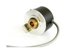
In the field of robotics, photoelectric encoder is usually used to measure the wheel speed. When the wheel rotates, the photoelectric encoder receives the pulse signal, which can be obtained by multiplying the number of pulses by the coefficient
Know how many turns the wheel has made.
The two wheeled robot can know how much the robot has advanced through the continuous integral operation of the wheel speed. At the same time, it can use the difference between the two wheel speeds to calculate the rotation of the robot
How many degrees, so as to realize the dead reckoning and positioning of the robot's track.
Relationship between wheel odometer and laser SLAM
One of the steps of laser SLAM for inter frame matching is to obtain the relative pose of the two moments through the point cloud matching of the two moments.
As mentioned above, the wheel odometer can also calculate the pose of the robot by counting the speed of the motor
Since the pose can be obtained, it involves the problem of multi-sensor fusion. When it comes to fusion, each sensor must have its own advantages and disadvantages
Laser SLAM is not applicable when there are few environmental geometric feature points, such as in the case of long corridor. Obviously, the wheel odometer has nothing to do with this situation
The wheel odometer will have cumulative error in case of road slip, which is obviously not the case in laser SLAM Since the two have their own strengths, they should be integrated
The idea of integration is as follows:
The positioning of wheel odometer can provide the initial value matching between two times for laser SLAM. When the initial value is accurate, the accuracy of laser SLAM can be improved.
In addition, the wheel odometer can realize short-range track dead reckoning and positioning alone, and the laser SLAM can also realize positioning. The integration of the two can enhance the accuracy of positioning
Robustness and robustness
Calibration of wheel odometer
The basic principle of wheel odometer is to use the difference between the speeds of two wheels to calculate how many degrees the robot has turned. This premise is that the wheel radius and the distance between the two wheels are known.
Therefore, in the following cases, it is necessary to calibrate the wheel odometer
- Wheel speedometer hardware deformation
- The wheel radius and the distance between the two wheels change
- Inaccurate conversion coefficient from pulse signal to wheel speed
Calibration methods can be divided into two categories
- White box calibration: when the physical model of the sensor is known, the model-based method needs to be adopted
- Black box calibration: when you don't know the physical model of the sensor, you can try the direct linear method
Linear least squares
For the linear case
Ax=b
This case is divided into several cases according to the dimension of A matrix
m is the number of rows of a and n is the number of columns of A
- When m=n, the well posed equations have a unique solution
- When m < n, the underdetermined equations have infinite solutions
- When m > N, the overdetermined equations have usually no solutions
In engineering applications, there are usually many overdetermined cases, and the overdetermined cases usually have no solution, so there is a linear least squares, which is equivalent to seeking the second best solution, that is, the most similar solution of the solution
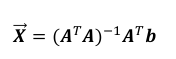
The formula of the general solution is
Odometer calibration by direct linear method
Core idea:
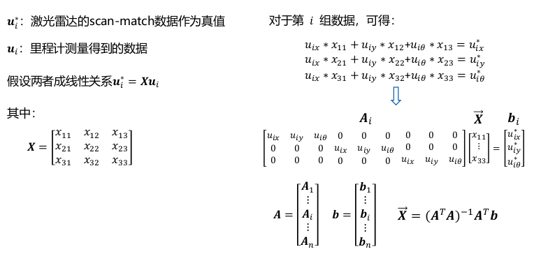
By collecting lidar data and wheel odometer data at the corresponding time, taking the pose difference of each frame of radar data as the true value, a transformation matrix is calculated to make the pose difference of wheel odometer after transformation equal to that of lidar data.
Corresponding mathematical model:
Code
With the above mathematical model, let's enter the code practice link
This paper focuses on the calibration of odometer, and uses the data of lidar to match the pose of ICP as the true value The processing of laser data in the code is not described in detail
int main(int argc,char** argv)
{

    ros::init(argc, argv, "Odom_Calib_node");
    ros::Time::init();
    ros::NodeHandle n;

    //Class object of instance Scan2
    Scan2 scan;
First, perform node initialization, handle declaration and other routine operations in the main function
Then the class object of instance Scan2
Let's look at Scan2's constructor
++++++++++++++++++++++++++++++++++++++++++++++++
//Constructor
Scan2::Scan2()
{
    //Declaration handle
    ros::NodeHandle private_nh_("~");

    //Laser data processing content
    m_prevLDP = NULL;
    SetPIICPParams();//Set PI_ICP parameters

    scan_pos_cal.setZero();//Laser data pose reset
    odom_pos_cal.setZero();//Odometer data pose reset
    odom_increments.clear();//It is used to store the incremental reset between two frames of odometer

    //Set coordinate system name
    if(!private_nh_.getParam("odom_frame", odom_frame_))
        odom_frame_ = "odom";
    if(!private_nh_.getParam("base_frame", base_frame_))
        base_frame_ = "base_link";

    //Subscribe to the corresponding topic, and the system will start the least squares solution after receiving the topic. Therefore, after the node receives enough data, it will start the solution after publishing a topic artificially
    calib_flag_sub_ = node_.subscribe("calib_flag",5,&Scan2::CalibFlagCallBack,this);

    //Handle to the publish path
    odom_path_pub_ = node_.advertise<nav_msgs::Path>("odom_path_pub_",1,true);//Wheel odometer path
    scan_path_pub_ = node_.advertise<nav_msgs::Path>("scan_path_pub_",1,true);//Laser path
    calib_path_pub_ = node_.advertise<nav_msgs::Path>("calib_path_pub_",1,true);//Corrected path
    current_time = ros::Time::now();

    path_odom.header.stamp=current_time;
    path_scan.header.stamp=current_time;
    path_odom.header.frame_id="odom";
    path_scan.header.frame_id="odom";

    //Synchronize odometer and lidar data through message_ Filter method for time synchronization
    scan_filter_sub_ = new message_filters::Subscriber<sensor_msgs::LaserScan>(node_, "/sick_scan", 10);
    scan_filter_ = new tf::MessageFilter<sensor_msgs::LaserScan>(*scan_filter_sub_, tf_, odom_frame_, 10);
    scan_filter_->registerCallback(boost::bind(&Scan2::scanCallBack, this, _1));

    std::cout <<"Calibration Online,Wait for Data!!!!!!!"<<std::endl;
}
Basic content annotated
Mainly do the initialization of related variables
Set the handle of subscription and publication topic
Finally, through message_ The method of filters is used for time synchronization of odometer and lidar data
Now you can see the callback function scanCallBack
++++++++++++++++++++++++++++++++++++++++++++++++
//Laser data callback function
void Scan2::scanCallBack(const sensor_msgs::LaserScan::ConstPtr &_laserScanMsg)
{
    static long int dataCnt = 0;
    sensor_msgs::LaserScan scan;
    Eigen::Vector3d odom_pose;              //Position and attitude of odometer corresponding to laser
    Eigen::Vector3d d_point_odom;           //dpose for odometer calculation
    Eigen::Vector3d d_point_scan;           //dpose calculated by scanmatch of laser
    Eigen::MatrixXd transform_matrix(3,3);  //Temporary variable

    double c,s;//cos and sin
    scan = *_laserScanMsg;//Get this frame data

    //Get the corresponding odometer data
    if(!getOdomPose(odom_pose, _laserScanMsg->header.stamp))
        return ;

    //Position and attitude difference of odometer in front and back frames
    d_point_odom = cal_delta_distence(odom_pose);
See here first. Only a few variables are generated here. The corresponding meanings of variables have been annotated
Find the corresponding odometer pose according to the time of the frame of the laser data. Note that this pose is in the world coordinate system
Then pass * cal_ delta_ The distance () function calculates the pose difference with the previous wheel odometer data
**Note: * * since the pose of the wheel odometer is in the world coordinate system, the pose difference is also the pose difference in the world coordinate system
However, the pose difference calculated from the laser data is in the coordinate system where the laser data of the previous frame is the origin, so the two pose differences calculated directly do not match
So in CAL_ delta_ In the distance() function, you need to convert the pose difference in the world coordinate system to the pose difference in the previous frame coordinate system
It's easy to ignore here
++++++++++++++++++++++++++++++++++++++++++++++++
Let's look at Cal first_ delta_ Distance() * function
//The pose difference between two frames of data is solved
//That is to solve the coordinates of the current pose in the previous coordinate system
Eigen::Vector3d  cal_delta_distence(Eigen::Vector3d odom_pose)
{
    Eigen::Vector3d d_pos;  //return value
    now_pos = odom_pose;

    /*Method 1: solve by coordinate transformation matrix */
    double c = cos(now_pos(2));//Calculate cos
    double s = sin(now_pos(2));//Calculate sin
    //Pose transformation matrix of the current time in the world coordinate system
    Eigen::Matrix3d TWN;
    TWN <<c,-s,now_pos(0),
          s, c,now_pos(1),
          0, 0,1;
     c = cos(last_pos(2));
     s = sin(last_pos(2));
    //Pose transformation matrix in the world coordinate system at the last time
    Eigen::Matrix3d TWL;
    TWL<<c,-s,last_pos(0),
         s, c,last_pos(1),
         0, 0,1;
    Eigen::Matrix3d TLN = TWL.inverse()*TWN;//Find the coordinate transformation matrix from the current time to the previous time

    d_pos << TLN(0,2),TLN(1,2),atan2(TLN(1,0),TLN(0,0));//Assignment coordinate transformation matrix, i.e. pose difference

    /*Method 2: turn the world coordinate system vector to the previous time coordinate system */
    /*
    d_pos=TWL.inverse()*( now_pos- last_pos);//It is equivalent to a deviation vector in the world coordinate system turning to the previous time coordinate system
    */
    /*Method 3: the method is the same as method 2, except that the rotation axis is used */
    /*
    Eigen::AngleAxisd temp(last_pos(2),Eigen::Vector3d(0,0,1));
    Eigen::Matrix3d trans=temp.matrix().inverse();
    d_pos=trans*(now_pos- last_pos);
    */

    return d_pos;
}
Three calculation methods are written here:
Method 1: solve by coordinate transformation matrix
Calculate the transformation matrix from the current pose to the world coordinate system according to the current pose, and calculate the transformation matrix from the previous frame to the world coordinate system according to the pose of the previous frame
Then, through the two transformation matrices, the coordinate transformation matrix from the current time to the previous time can be calculated, and this transformation matrix can be converted into pose difference
Method 2: turn the world coordinate system vector to the previous time coordinate system
It is equivalent to a deviation vector in the world coordinate system turning to the previous time coordinate system
Method 3: the method is the same as method 2, except that the rotation axis is used

The pose difference of a frame of data printed
Next, continue to return to the laser data callback function
++++++++++++++++++++++++++++++++++++++++++++++++
    //If the distance of movement is too short, no processing is carried out
    if(d_point_odom(0) < 0.05 &&
       d_point_odom(1) < 0.05 &&
       d_point_odom(2) < tfRadians(5.0))
    {
        return ;
    }
If the distance of movement is too short, no processing is carried out
    last_pos = now_pos;//Save the current pose as the pose iteration of the previous frame
        //Record the incremental data of the odometer
    odom_increments.push_back(d_point_odom);
    //Convert the current laser data into the data recognized by PL ICP for correction
    //d_point_scan is the rotation translation between two frames of data calculated by laser
    LDP currentLDP;
    if(m_prevLDP != NULL)
    {
        LaserScanToLDP(&scan,currentLDP);
        d_point_scan = PIICPBetweenTwoFrames(currentLDP,d_point_odom);
    }
    else
    {
        LaserScanToLDP(&scan,m_prevLDP);
    }
Convert the current laser data into the data recognized by PL ICP for correction
d_point_scan is the rotation translation between two frames of data calculated by laser
The processing part of laser data is not detailed
    // Two needle scan calculates the accumulated pose of itself for laser_path visualization
    c = cos(scan_pos_cal(2));
    s = sin(scan_pos_cal(2));
    transform_matrix<<c,-s,0,
                      s, c,0,
                      0, 0,1;
    scan_pos_cal+=(transform_matrix*d_point_scan);

    // Odometer accumulated pose for odom_path visualization
    c = cos(odom_pos_cal(2));
    s = sin(odom_pos_cal(2));
    transform_matrix<<c,-s,0,
                      s, c,0,
                      0, 0,1;
    odom_pos_cal+=(transform_matrix*d_point_odom);

    //Put in the path / / for visualization
    pub_msg(odom_pos_cal,path_odom,odom_path_pub_);
    pub_msg(scan_pos_cal,path_scan,scan_path_pub_);
The direct errors of the two frames calculated by the laser are accumulated into the pose in world coordinates, and then the path is released for viewing in rviz
Similarly, the direct error of two frames calculated by the wheel odometer is accumulated into the position and attitude in the world coordinates, and then the path is released for viewing in rviz
    //Constructing overdetermined equations
    Odom_calib.Add_Data(d_point_odom,d_point_scan);

    //Quantity for calibration
    dataCnt++;

    std::cout <<"Data Cnt:"<<dataCnt<<std::endl;//Amount of data for terminal output
Add two pose differences to the equations
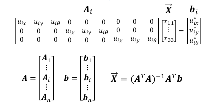
It is this equation that Ai is the odometer pose data of one frame, and A is all odometer pose data
bi is one frame of lidar pose data, and b is all lidar pose data
So in add_ In the data() function, each frame of data needs to be combined into A matrix and b matrix
++++++++++++++++++++++++++++++++++++++++++++++++
Let's look at add_ Implementation of data() function
bool OdomCalib::Add_Data(Eigen::Vector3d Odom,Eigen::Vector3d scan)
{

    if(now_len<INT_MAX)
    {
        /*Construction matrix A*/
        Eigen::MatrixXd Ai;//A matrix of the ith degree
        Ai.resize(3,9); //Initialize Ai size
        //Assignment AI
        Ai<<Odom(0),Odom(1),Odom(2),0,0,0,0,0,0,
            0,0,0, Odom(0),Odom(1),Odom(2),0,0,0,
            0,0,0,0,0,0,Odom(0),Odom(1),Odom(2);

        Eigen::Vector3d  bi;//b vector of the i th degree
        bi<<scan(0),scan(1),scan(2);//Assignment bi

        if(now_len==0)
        {   //First data
            A.resize(3,9);
            A =  Ai;
            b.resize(3,1);
            b=bi;
        }else{
            A.conservativeResize(3+3*now_len,9);//Redefine the size of A matrix without changing the original value. The difference between conservative resize and resize is whether to initialize the original value
            A.block<3,9>(3*now_len,0)=Ai;//Overlay on specified block
            b.conservativeResize(3+3*now_len,1);//Redefine the size of the b matrix without changing the original value
            b.block<3,1>(3*now_len,0)=bi;//Overlay on specified block
        }
        //std::cout <<"A: "<<std::endl;
        //std::cout <<A<<std::endl;// Printout a
        //std::cout <<"b: "<<std::endl;
        //std::cout <<b<<std::endl;// Printout A
        now_len++;
        return true;
    }
    else
    {
        return false;
    }
}
Firstly, Ai and bi are constructed by odometer pose and lidar pose corresponding to formal parameters
Then continue to add corresponding matrices to A and b
The matrix of eigen is added without the convenience of opencv, and there is no specific function. The method used here is
Declaring dynamic matrix A means not specifying the size of A, and then setting the matrix size through * conservatoresize() function when adding,
Note that the difference between this function and resize() * is whether to save the previous value. If resize, it will all become 0
Then you can add it to the specified block through the block module of eigen
A matrix is continuously added, and the result is as follows:
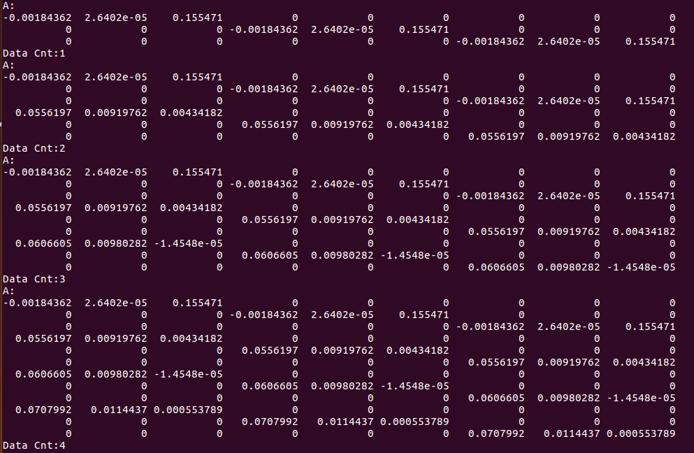
The b matrix is like this
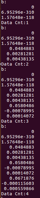
So far, A steady stream of data comes in, and then A and b gradually add their own matrix data, and the mathematical equation is constructed
Then it can be solved by the corresponding formula
It's this formula. We know A and b to find X
++++++++++++++++++++++++++++++++++++++++++++++++
Previously, a subscription topic was declared in the constructor of Scan2()
Will subscribe to "calib_flag"
After the node is running, it receives enough data and manually publishes a topic to start the solution
The program enters the * CalibFlagCallBack() * callback function
//Subscribing to topic means starting calibration
void Scan2::CalibFlagCallBack(const std_msgs::Empty &msg)
{
    //Linear least squares solution
    Eigen::Matrix3d correct_matrix = Odom_calib.Solve();

    Eigen::Matrix3d tmp_transform_matrix;

    std::cout<<"correct_matrix:"<<std::endl<<correct_matrix<<std::endl;

    //Calculate the corrected path
    Eigen::Vector3d calib_pos(0,0,0);                 //Corrected posture
    std::vector<Eigen::Vector3d> calib_path_eigen;    //Corrected path
    for(int i = 0; i < odom_increments.size();i++)
    {
        Eigen::Vector3d odom_inc = odom_increments[i];//Position and attitude difference of odometer this time
        Eigen::Vector3d correct_inc = correct_matrix * odom_inc;//Correct the posture difference

        tmp_transform_matrix << cos(calib_pos(2)),-sin(calib_pos(2)),0,
                            sin(calib_pos(2)), cos(calib_pos(2)),0,
                                            0,                 0,1;

        calib_pos += tmp_transform_matrix * correct_inc;//Corrected pose in cumulative world coordinate system

        calib_path_eigen.push_back(calib_pos);//Constitute path
    }

    //Path after publishing correction
    publishPathEigen(calib_path_eigen,calib_path_pub_);

    //After correction, exit the subscription
    scan_filter_sub_->unsubscribe();

    std::cout <<"calibration over!!!!"<<std::endl;
}
First, solve the linear least squares by * Solve()
Then, correct the pose difference of each odometer frame, and then turn to the world coordinate system to accumulate continuously to form a path, and finally release the corrected path
++++++++++++++++++++++++++++++++++++++++++++++++
Finally, let's take a look at how the * Solve() * function performs the linear least squares solution
/*
 * Solving linear least squares Ax=b
 * Return the obtained correction matrix
*/
Eigen::Matrix3d OdomCalib::Solve()
{
    Eigen::Matrix3d correct_matrix;
    /*Method 1: solve according to the least square formula*/
    //The solution vector is obtained by solving the linear least square formula
    Eigen::Matrix<double,9,1> correct_vector = (A.transpose()*A).inverse()*A.transpose()*b;
    //Assignment correction matrix
    correct_matrix << correct_vector(0),correct_vector(1),correct_vector(2),
                      correct_vector(3),correct_vector(4),correct_vector(5),
                      correct_vector(6),correct_vector(7),correct_vector(8);
    /*Method 2: solve by matrix QR decomposition*/
    /*
    correct_vector = A.colPivHouseholderQr().solve(b);
        correct_matrix << correct_vector(0),correct_vector(1),correct_vector(2),
                      correct_vector(3),correct_vector(4),correct_vector(5),
                      correct_vector(6),correct_vector(7),correct_vector(8);
    */


    return correct_matrix;
}
Method 1: solve according to the least square formula
Method 2: solve by matrix QR decomposition
++++++++++++++++++++++++++++++++++++++++++++++++
Result
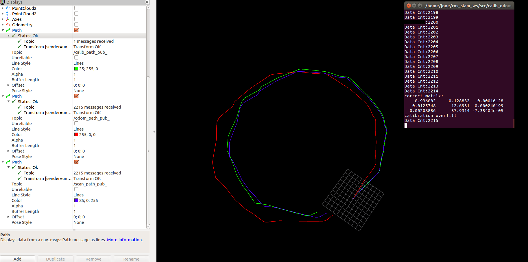
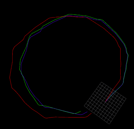
Red is the odometer path, blue is the lidar path, and green is the calibrated path.
You can see that after calibration, it is closer to the laser radar path

Matrix obtained after calibration