1, Introduction to image denoising and filtering
1 image denoising
1.1 definition of image noise
Noise is an important factor that interferes with the visual effect of image. Image denoising refers to the process of reducing noise in image. There are three kinds of noise classification: additive noise, multiplicative noise and quantization noise. We use f(x,y) to represent the image, g(x,y) to represent the image signal, and n(x,y) to represent the noise.
Image denoising refers to the process of reducing noise in digital images. The digital image in reality is often affected by the noise interference of imaging equipment and external environment in the process of digitization and transmission, which is called noisy image or noisy image. Denoising is an important content in image processing. In the process of image acquisition, transmission, transmission, reception, replication and output, noise is often generated. Salt and pepper noise is a common noise, which belongs to additive noise.
1.2 image noise source
(1) During image acquisition
In the process of image acquisition by CCD and CMOS image sensors, various noises will be introduced due to the influence of sensor material properties, working environment, electronic components and circuit structure.
(2) During image signal transmission
Due to the imperfection of transmission media and recording equipment, digital images are often polluted by a variety of noise in the process of transmission and recording.
1.3 noise classification
Noise can be classified in different forms according to different classification standards:
Based on the causes: internal noise, external noise.
Based on the relationship between noise and signal:
Additive noise: additive noise is not related to image signal strength. This kind of noisy image g can be regarded as the sum of ideal noise free image f and noise n:
g = f + n;
Multiplicative voice: multiplicative noise is related to the image signal and often changes with the change of the image signal. The noise generated by the change of the carrier carrying each pixel information is modulated by the information itself. In some cases, for example, the signal change is small and the noise is small. For the convenience of analysis and processing, multiplicative noise is often regarded as additive noise, and it is always assumed that signal and noise are statistically independent of each other.
g = f + f*n
According to the probability density function based on Statistics:
It is more important, mainly because the introduction of mathematical model is helpful to remove noise by mathematical means. In different scenes, the application methods of noise are different. Because under certain external conditions, the probability density function (statistical result) of the image original image under noise (without noise) obeys a certain distribution function, it is classified as the corresponding noise. The noise classification based on the statistical probability density function and its elimination method will be described in detail below.
1.4 classification of image denoising algorithms
(1) Spatial domain filtering
Spatial filtering is to directly perform data operation on the original image and process the gray value of pixels. Common spatial domain image denoising algorithms include neighborhood average method, median filter, low-pass filter and so on.
(2) Transform domain filtering
The image transform domain denoising method is to transform the image from the spatial domain to the transform domain, process the transform coefficients in the transform domain, and then inverse transform the image from the transform domain to the spatial domain to remove the image noise. There are many methods to transform images from spatial domain to transform domain, such as Fourier transform, Walsh Hadamard transform, cosine transform, K-L transform and wavelet transform. Fourier transform and wavelet transform are common transform methods for image denoising.
(3) Partial differential equation
Partial differential equation is an image processing method rising in recent years. It mainly aims at low-level image processing and has achieved good results. Partial differential equation has the characteristics of anisotropy. When applied in image denoising, it can remove noise and maintain the edge well. The application of partial differential equations can be divided into two categories: one is the basic iterative format, which makes the image gradually approach the desired effect through the update over time. The representative of this algorithm is Perona and Malik's equations, and the follow-up work after its improvement. This method has a large selection space in determining the diffusion coefficient. It has the function of backward diffusion while forward diffusion. Therefore, it has the ability to smooth the image and sharpen the edge. Partial differential equations have achieved good results in image processing with low noise density, but the denoising effect is not good when processing images with high noise density, and the processing time is much higher.
(4) Variational method
Another image denoising method using mathematics is to determine the energy function of the image based on the idea of variational method, and make the image reach a smooth state by minimizing the energy function. The fully variational TV model which is widely used now is this kind. The key of this kind of method is to find an appropriate energy equation to ensure the stability of evolution and obtain ideal results.
Morphological noise filter can be used to filter noise by combining open and close. Firstly, the noisy image can be opened, and the structure element matrix can be selected to be larger than the noise size. Therefore, the result of open operation is to remove the background noise; Then close the image obtained in the previous step to remove the noise on the image. Therefore, it can be seen that the image type applicable to this method is that the object size in the image is relatively large and there are no small details, so the denoising effect of this kind of image will be better.
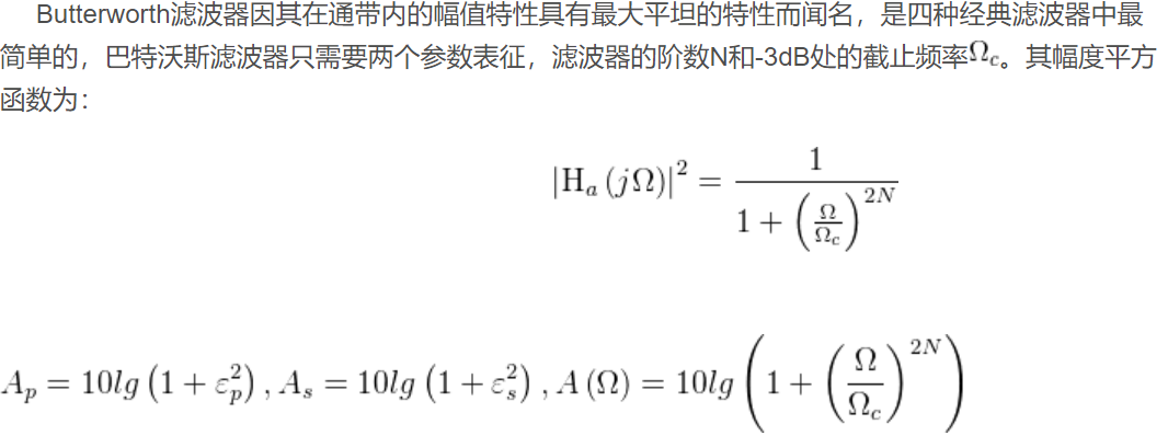
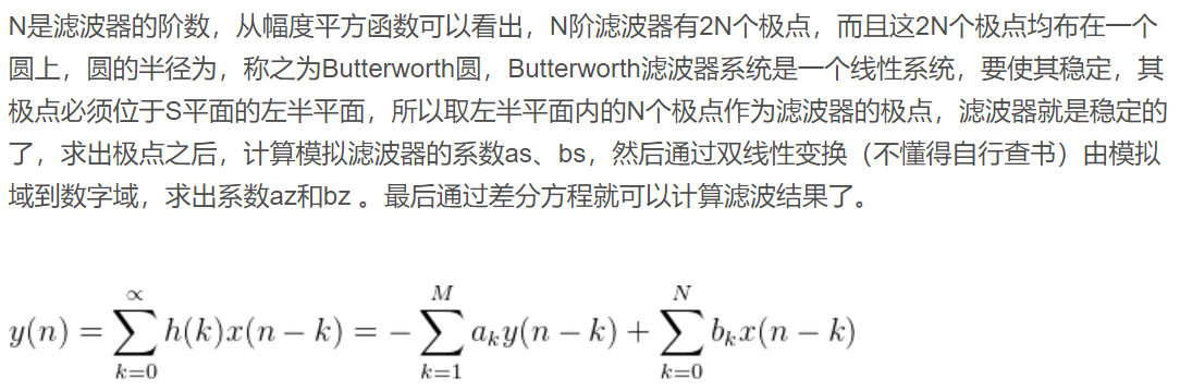
2 butterworth
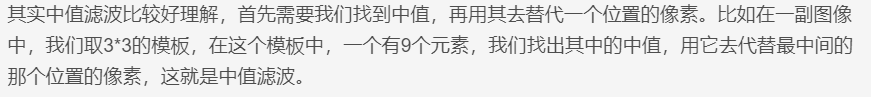
3 median filtering
(1) Concept:
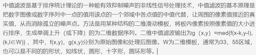
(2) Principle explanation:
4-wiener filtering
Wiener filtering is an optimal estimator for stationary processes based on the minimum mean square error criterion. The mean square error between the output of this filter and the expected output is the smallest, so it is an optimal filtering system. It can be used to extract signals contaminated by stationary noise.
5 wavelet filtering
With the increasing improvement of wavelet theory, it has attracted more and more attention in the field of image denoising with its good time-frequency characteristics, which opens up the precedent of denoising with nonlinear methods. Specifically, wavelet denoising is mainly due to the following characteristics of wavelet transform:
(1) Low entropy. The sparse distribution of wavelet coefficients reduces the entropy after image transformation. It means that after the signal (i.e. image) is decomposed, more wavelet base coefficients tend to 0 (noise), and the main parts of the signal are mostly concentrated in some wavelet bases. Using threshold denoising can better retain the original signal.
(2) Multi resolution characteristics. Due to the multi-resolution method, the nonstationarity of the signal can be well characterized, such as mutation and breakpoint (for example, 0-1 mutation cannot be reasonably represented by Fourier change). The noise can be eliminated according to the distribution of signal and noise at different resolutions.
(3) Decorrelation. Wavelet transform can decorrelate the signal, and the noise tends to whiten after transform, so wavelet domain is more conducive to denoising than time domain.
(4) Flexible selection of basis functions. Wavelet transform can flexibly select the basis function, multi band wavelet and wavelet packet can also be selected according to the signal characteristics and denoising requirements (wavelet packet decomposes the high-frequency signal again to improve the time-frequency resolution), and different wavelet basis functions can be selected for different occasions.
According to different processing methods based on wavelet coefficients, common denoising methods can be divided into three categories:
(1) Denoising based on wavelet transform modulus maxima (signal and noise modulus maxima will show different trends under wavelet transform)
(2) Denoising based on the correlation of wavelet coefficients of adjacent scales (noise has no obvious correlation among wavelet transform scales, while signal has the opposite)
(3) Threshold denoising based on Wavelet Transform
Implementation steps of wavelet denoising:
(1) Wavelet decomposition of two-dimensional signal. Select a wavelet and wavelet decomposition level N, and then calculate the decomposition of signal s to level N.
(2) Threshold quantization of high frequency coefficients. For each layer from 1 to N, a threshold is selected, and the high-frequency coefficients of this layer are soft threshold quantized.
(3) Two dimensional wavelet reconstruction. According to the low-frequency coefficients of the nth layer of wavelet decomposition and the modified high-frequency coefficients of each layer from the first layer to the nth layer, the wavelet reconstruction of two-dimensional signal is calculated.
2, Partial source code
function varargout = GUI_3(varargin)
% GUI_3 MATLAB code for GUI_3.fig
% GUI_3, by itself, creates a new GUI_3 or raises the existing
% singleton*.
%
% H = GUI_3 returns the handle to a new GUI_3 or the handle to
% the existing singleton*.
%
% GUI_3('CALLBACK',hObject,eventData,handles,...) calls the local
% function named CALLBACK in GUI_3.M with the given input arguments.
%
% GUI_3('Property','Value',...) creates a new GUI_3 or raises the
% existing singleton*. Starting from the left, property value pairs are
% applied to the GUI before GUI_3_OpeningFcn gets called. An
% unrecognized property name or invalid value makes property application
% stop. All inputs are passed to GUI_3_OpeningFcn via varargin.
%
% *See GUI Options on GUIDE's Tools menu. Choose "GUI allows only one
% instance to run (singleton)".
%
% See also: GUIDE, GUIDATA, GUIHANDLES
% Edit the above text to modify the response to help GUI_3
% Last Modified by GUIDE v2.5 27-Apr-2013 11:43:14
% Begin initialization code - DO NOT EDIT
gui_Singleton = 1;
gui_State = struct('gui_Name', mfilename, ...
'gui_Singleton', gui_Singleton, ...
'gui_OpeningFcn', @GUI_3_OpeningFcn, ...
'gui_OutputFcn', @GUI_3_OutputFcn, ...
'gui_LayoutFcn', [] , ...
'gui_Callback', []);
if nargin && ischar(varargin{1})
gui_State.gui_Callback = str2func(varargin{1});
end
if nargout
[varargout{1:nargout}] = gui_mainfcn(gui_State, varargin{:});
else
gui_mainfcn(gui_State, varargin{:});
end
% End initialization code - DO NOT EDIT
% --- Executes just before GUI_3 is made visible.
function GUI_3_OpeningFcn(hObject, eventdata, handles, varargin)
% This function has no output args, see OutputFcn.
% hObject handle to figure
% eventdata reserved - to be defined in a future version of MATLAB
% handles structure with handles and user data (see GUIDATA)
% varargin command line arguments to GUI_3 (see VARARGIN)
% Choose default command line output for GUI_3
handles.output = hObject;
% Update handles structure
guidata(hObject, handles);
% UIWAIT makes GUI_3 wait for user response (see UIRESUME)
% uiwait(handles.figure1);
% --- Outputs from this function are returned to the command line.
function varargout = GUI_3_OutputFcn(hObject, eventdata, handles)
% varargout cell array for returning output args (see VARARGOUT);
% hObject handle to figure
% eventdata reserved - to be defined in a future version of MATLAB
% handles structure with handles and user data (see GUIDATA)
% Get default command line output from handles structure
varargout{1} = handles.output;
% --- Executes on button press in pushbutton1.
function pushbutton1_Callback(hObject, eventdata, handles)
% hObject handle to pushbutton1 (see GCBO)
% eventdata reserved - to be defined in a future version of MATLAB
% handles structure with handles and user data (see GUIDATA)
global im
global x
%Select picture path
[filename, pathname]= ...
uigetfile({'*.jpg';'*.bmp';'*.gif'},'Select Picture');
%Synthetic path+file name
str=[pathname filename];
%Read picture
im=imread(str);
%Use first axes
axes(handles.axes1);
%display picture
imshow(im);
axes(handles.axes5);
imshow(im);
% --- Executes on button press in pushbutton2.
function pushbutton2_Callback(hObject, eventdata, handles)
% hObject handle to pushbutton2 (see GCBO)
% eventdata reserved - to be defined in a future version of MATLAB
% handles structure with handles and user data (see GUIDATA)
close(gcf)
% --- Executes when selected object is changed in uipanel1.
function uipanel1_SelectionChangeFcn(hObject, eventdata, handles)
% hObject handle to the selected object in uipanel1
% eventdata structure with the following fields (see UIBUTTONGROUP)
% EventName: string 'SelectionChanged' (read only)
% OldValue: handle of the previously selected object or empty if none was selected
% NewValue: handle of the currently selected object
% handles structure with handles and user data (see GUIDATA)
global im
str=get(hObject,'string');
axes(handles.axes1);
switch str
case 'Original drawing'
imshow(im);
case 'sobel'
BW = edge(rgb2gray(im),'sobel');
imshow(BW);
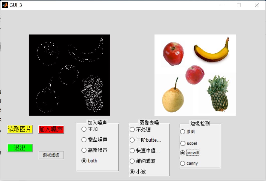
case 'prewitt'
BW = edge(rgb2gray(im),'prewitt');
imshow(BW);
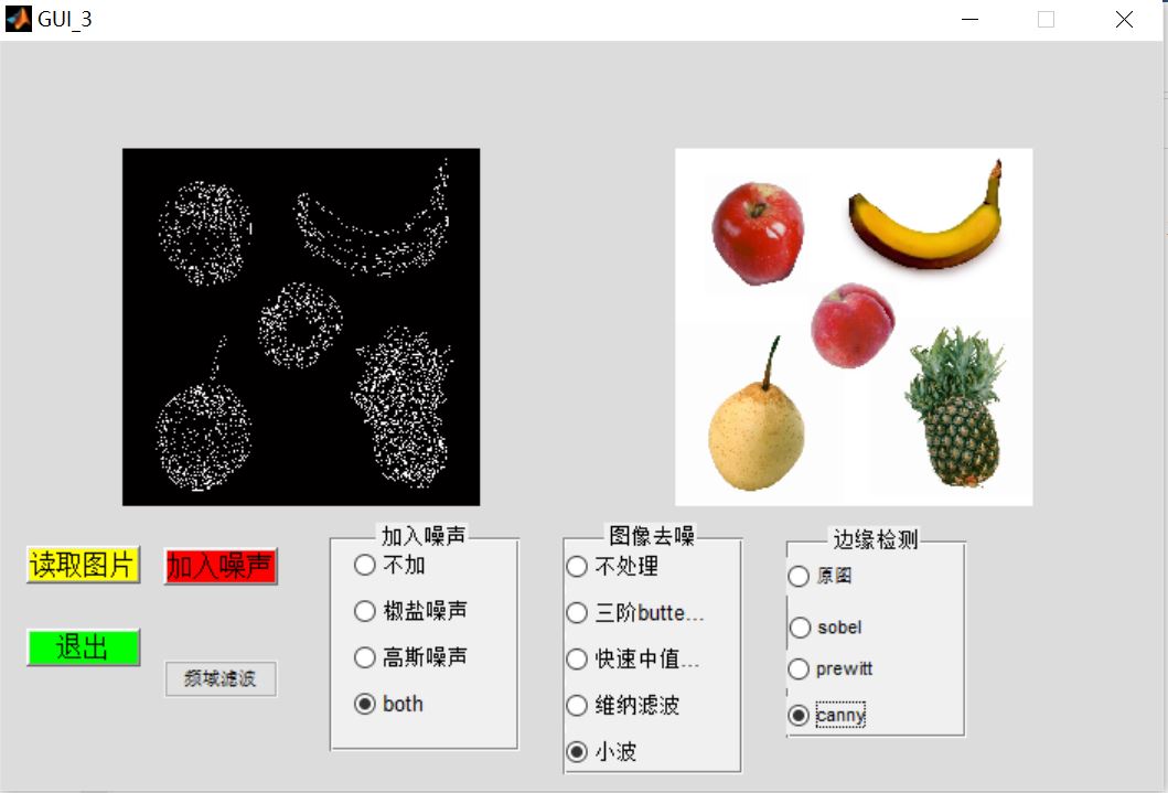
case 'canny'
BW = edge(rgb2gray(im),'canny');
imshow(BW);
end;
% --- Executes when selected object is changed in uipanel4.
function uipanel4_SelectionChangeFcn(hObject, eventdata, handles)
% hObject handle to the selected object in uipanel4
% eventdata structure with the following fields (see UIBUTTONGROUP)
% EventName: string 'SelectionChanged' (read only)
% OldValue: handle of the previously selected object or empty if none was selected
% NewValue: handle of the currently selected object
% handles structure with handles and user data (see GUIDATA)
global im
global X
str=get(hObject,'string');
axes(handles.axes1);
switch str
case 'No'
imshow(im);
case 'Salt and pepper noise'
load sinsin
X=imnoise(im,'salt & pepper',0.05);
imshow(X);
case 'Gaussian noise '
load sinsin
X=imnoise(im,'gaussian',0.05);
imshow(X);
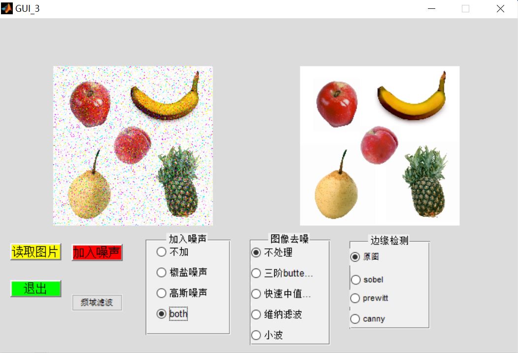
case 'both'
load sinsin
Y=imnoise(im,'salt & pepper',0.05);
X=imnoise(Y,'gaussian',0.05);
imshow(X);
end;
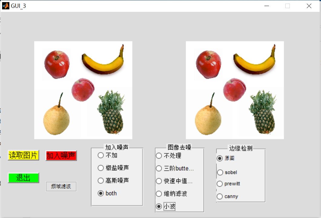
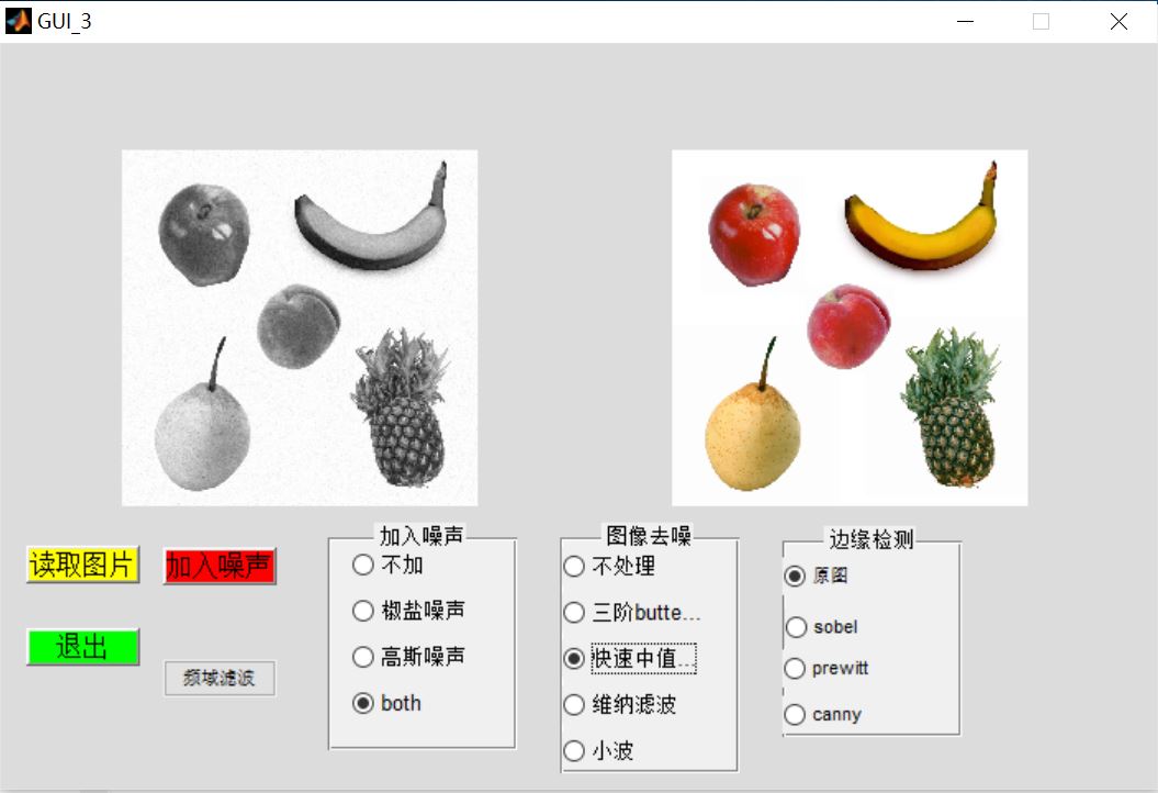
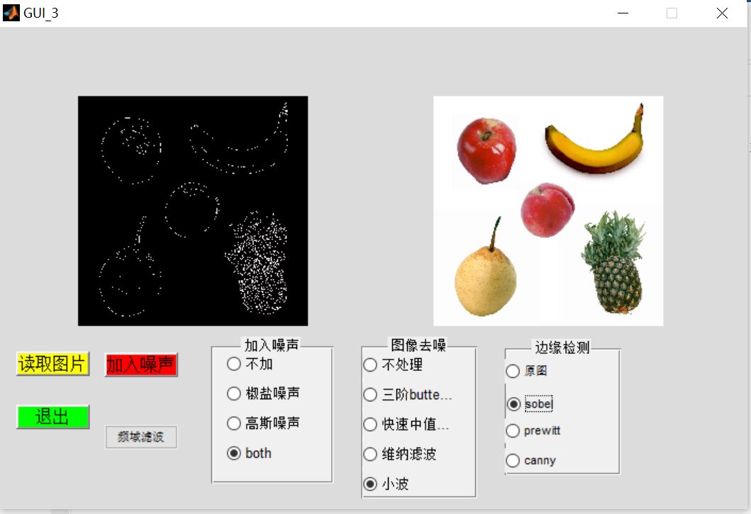
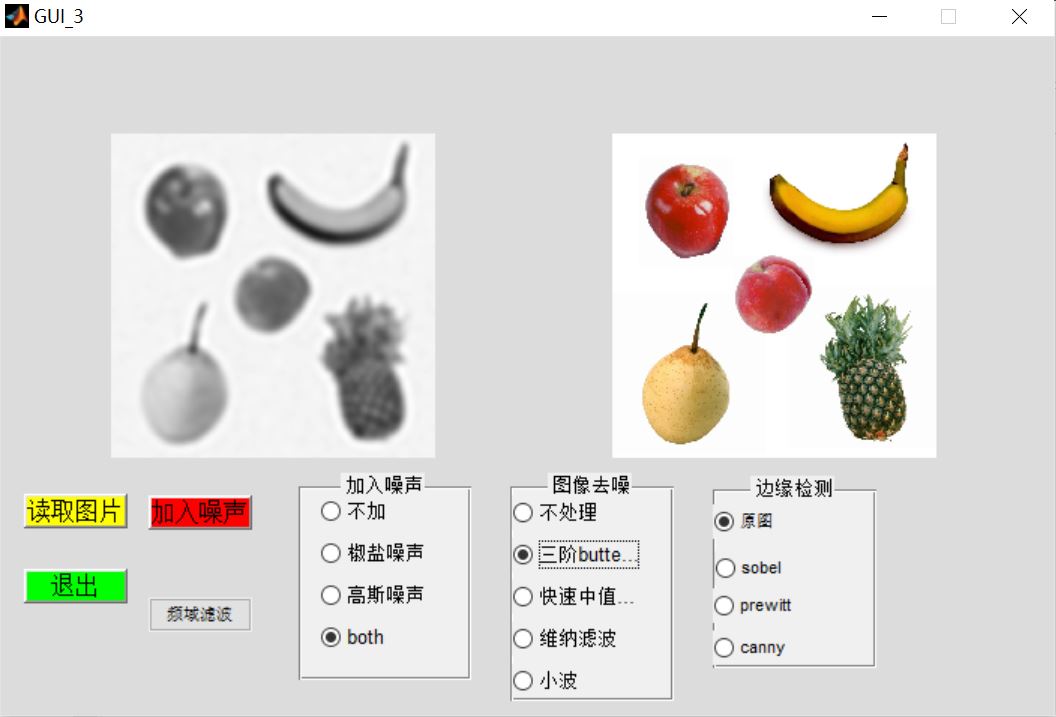
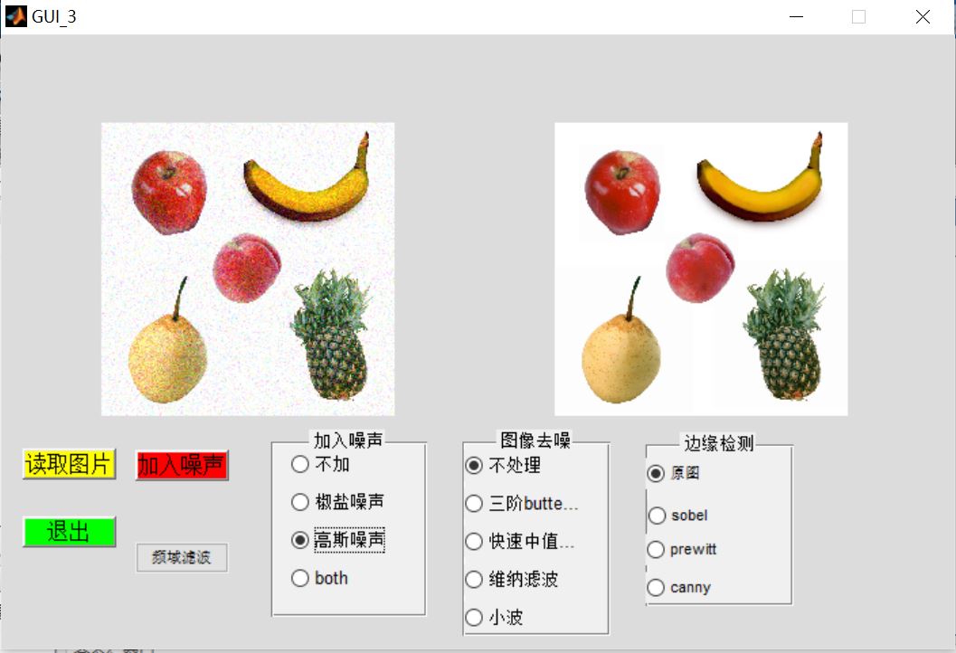
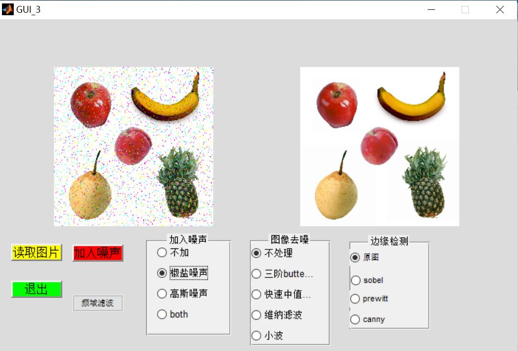
3, Operation results
4, matlab version and references
1 matlab version
2014a
2 references
[1] Cai Limei MATLAB image processing -- theory, algorithm and example analysis [M] Tsinghua University Press, 2020
[2] Yang Dan, Zhao Haibin, long Zhe Detailed explanation of MATLAB image processing example [M] Tsinghua University Press, 2013
[3] Zhou pin MATLAB image processing and graphical user interface design [M] Tsinghua University Press, 2013
[4] Liu Chenglong Proficient in MATLAB image processing [M] Tsinghua University Press, 2015
[5]Implementation principle of traditional image denoising algorithm based on matlab