Completed today: [100 OpenCV routines] 100 Adaptive local noise reduction filter
Celebration and change: Python white OpenCV learning class from scratch - 8 Frequency domain image filtering (I)
Welcome to pay attention "100 routines" Series, continuously updating
Welcome to pay attention "Python Xiaobai's OpenCV learning course" Series, continuously updating
Python white OpenCV learning class from scratch - 8 Frequency domain image filtering (I)
This series is for Python Xiaobai and explains the actual combat of OpenCV project from scratch.
The common operation of image preprocessing is to preserve the image features as much as possible.
Frequency domain image processing first carries out the Fourier transform of the image, then processes it in the transform domain, and finally carries out the inverse Fourier transform to transform it back to the spatial domain.
Frequency domain filtering is the multiplication of the filter transfer function and the corresponding pixel of the Fourier transform of the input image. The concept of filtering in frequency domain is more intuitive and the filter design is easier. Using fast Fourier transform algorithm is much faster than spatial convolution.
This paper provides the complete routines and running results of the above algorithms, and demonstrates the comprehensive use of a variety of image enhancement methods through an application case.
1. Fourier transform
Filtering usually refers to filtering or suppressing the components of a specific frequency in the image. Image filtering is a common image preprocessing operation to suppress the noise of the target image while preserving the detailed features of the image as much as possible.
Image filtering can be carried out not only in spatial domain, but also in frequency domain. Spatial filtering is the convolution between the image and various spatial filters (template and kernel), and the Fourier transform of spatial convolution is the product of the corresponding transform in the frequency domain. Therefore, frequency domain filtering is the multiplication of the frequency domain filter (transfer function) and the Fourier transform of the image.
In frequency domain image filtering, the image is first transformed by Fourier transform, then processed in the transform domain, and finally transformed back to the spatial domain by inverse Fourier transform.
The spatial domain filter and the frequency domain filter form a Fourier transform pair:
f
(
x
,
y
)
⊗
h
(
x
,
y
)
⇔
F
(
u
,
v
)
H
(
u
,
v
)
f
(
x
,
y
)
h
(
x
,
y
)
⇔
F
(
u
,
v
)
⊗
H
(
u
,
v
)
f(x,y) \otimes h(x,y) \Leftrightarrow F(u,v)H(u,v) \\f(x,y) h(x,y) \Leftrightarrow F(u,v) \otimes H(u,v)
f(x,y)⊗h(x,y)⇔F(u,v)H(u,v)f(x,y)h(x,y)⇔F(u,v)⊗H(u,v)
In other words, spatial domain filters and frequency domain filters are actually corresponding to each other. Some spatial domain filters will be more convenient and faster to realize by Fourier transform in frequency domain. For example, Laplace filter in spatial domain is a high pass filter in frequency domain.
1.1 Fourier series and Fourier transform
Fourier series is widely used in number theory, combinatorial mathematics, signal processing, probability theory, statistics, cryptography, acoustics, optics and other fields.
The Fourier series formula points out that any periodic function can be expressed as the weighted sum of sinusoidal and / or cosine functions of different frequencies:
f
(
t
)
=
A
0
+
∑
n
=
1
∞
A
n
s
i
n
(
n
ω
t
+
ψ
n
)
=
A
0
+
∑
n
=
1
∞
[
a
n
c
o
s
(
n
ω
t
)
+
b
n
s
i
n
(
n
ω
t
)
]
\begin{aligned} f(t) &= A_0 + \sum^{\infty}_{n=1} A_n sin(n \omega t + \psi _n)\\ &= A_0 + \sum^{\infty}_{n=1} [a_n cos(n \omega t) + b_n sin(n \omega t)] \end{aligned}
f(t)=A0+n=1∑∞Ansin(nωt+ψn)=A0+n=1∑∞[ancos(nωt)+bnsin(nωt)]
This sum is Fourier series.
Further, any aperiodic function can also be expressed as the integral of sine and / or cosine functions of different frequencies multiplied by the weighting function:
F
(
ω
)
=
∫
−
∞
+
∞
f
(
t
)
e
−
j
ω
t
d
t
f
(
t
)
=
1
2
π
∫
−
∞
+
∞
F
(
ω
)
e
j
ω
t
d
ω
\begin{aligned} F(\omega) &= \int_{-\infty}^{+\infty} f(t) e^{-j\omega t} dt\\ f(t) &= \frac{1}{2 \pi} \int_{-\infty}^{+\infty} F(\omega) e^{j\omega t} d \omega \end{aligned}
F(ω)f(t)=∫−∞+∞f(t)e−jωtdt=2π1∫−∞+∞F(ω)ejωtdω
This formula is Fourier transform and inverse transform.
*The sufficient condition for the existence of Fourier transform is that the integral of the absolute value of f(t) is limited, which can be satisfied in the fields of signal processing and image processing.
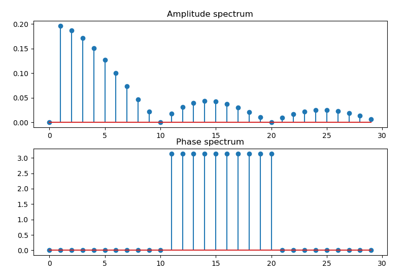
Routine 8.1: Fourier series of continuous periodic signals
    # 8.1: Fourier series of continuous periodic signal
    from scipy import integrate

    nf = 30
    T = 10
    tao = 1.0
    y = 1

    k = np.arange(0, nf)
    an = np.zeros(nf)
    bn = np.zeros(nf)
    amp = np.zeros(nf)
    pha = np.zeros(nf)

    half0, err0 = integrate.quad(lambda t: y, -tao/2, tao/2)
    an[0] = 2 * half0 / T
    for n in range(1, nf):
        half1, err1 = integrate.quad(lambda t: 2*y * np.cos(2.0/T * np.pi * n * t), -tao/2, tao/2)
        an[n] = half1 / 10
        half2, err2 = integrate.quad(lambda t: 2*y * np.sin(2.0/T * np.pi * n * t), -tao/2, tao/2)
        bn[n] = half2 / 10
        amp[n] = np.sqrt(an[n]**2 + bn[n]**2)

    for i in range(0, nf):
        pha[i] = 0.0 if an[i]>=0 else np.pi

    plt.figure(figsize=(9, 6))
    plt.subplot(211), plt.title("Amplitude spectrum"), plt.stem(k, amp)
    plt.subplot(212), plt.title("Phase spectrum"), plt.stem(k, pha)
    plt.show()
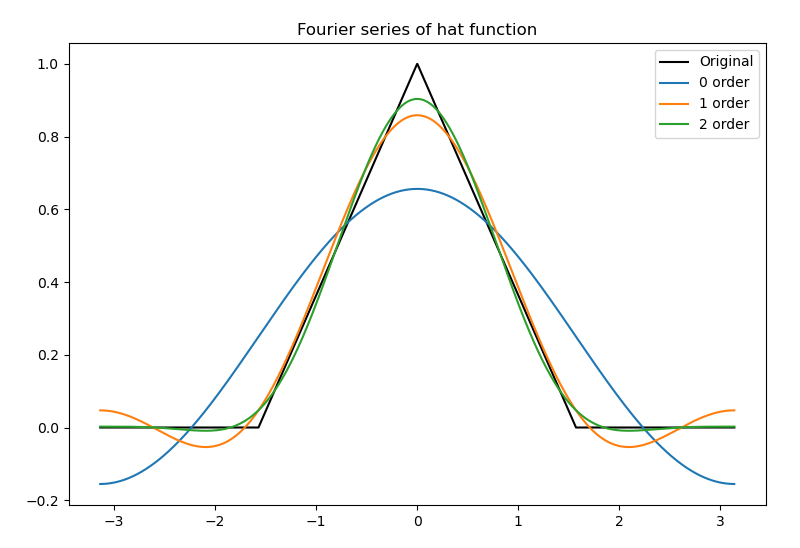
Routine 8.2: Fourier coefficients of continuous aperiodic signals
    # 8.2: Fourier coefficients of continuous aperiodic signals
    dx = 0.001
    x = np.pi * np.arange(-1+dx, 1+dx, dx)
    n = len(x)
    nquart = int(np.floor(n/4))

    f = np.zeros_like(x)
    f[nquart: 2*nquart] = (4/n) * np.arange(1, nquart+1)
    f[2*nquart: 3*nquart] = np.ones(nquart) - (4/n) * np.arange(0, nquart)

    plt.figure(figsize=(9, 6))
    plt.title("Fourier series of hat function")
    plt.plot(x, f, '-', color='k',label="Original")

    # Compute Fourier series
    A0 = np.sum(f * np.ones_like(x)) * dx
    fFS = A0 / 2

    orders = 3
    A = np.zeros(orders)
    B = np.zeros(orders)
    for k in range(orders):
        A[k] = np.sum(f * np.cos(np.pi * (k+1) * x / np.pi)) * dx  # Inner product
        B[k] = np.sum(f * np.sin(np.pi * (k+1) * x / np.pi)) * dx
        fFS = fFS + A[k] * np.cos((k + 1) * np.pi * x / np.pi) + B[k] * np.sin((k + 1) * np.pi * x / np.pi)

        plt.plot(x, fFS, '-', label="{} order".format(k))
        print('Line ', k, ': A = ', A[k], ' B = ', B[k], fFS.shape)

    plt.legend(loc="upper right")
    plt.show()
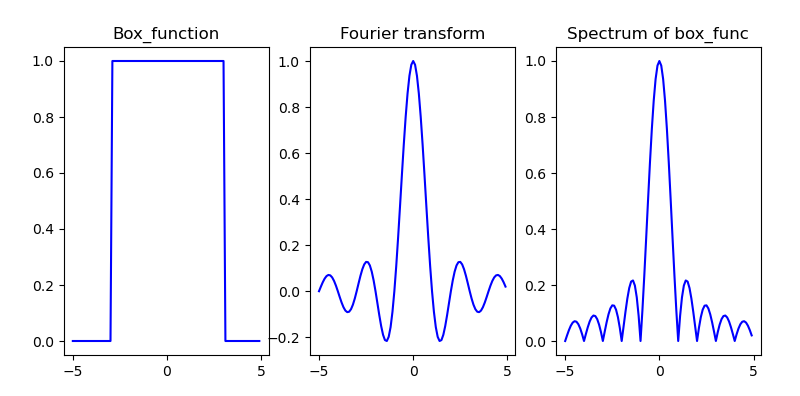
Routine 8.3: Fourier transform of one-dimensional continuous function (box function)
Taking one-dimensional box function as an example, its Fourier transform is:
F ( ω ) = ∫ − ∞ + ∞ f ( t ) e − j ω t d t = ∫ − π π f ( t ) e − j ω t d t = s i n ( ω ) ω \begin{aligned} F(\omega) &= \int_{-\infty}^{+\infty} f(t) e^{-j\omega t} dt\\ &= \int_{-\pi}^{\pi} f(t) e^{-j\omega t} dt\\ &= \frac{sin(\omega)}{\omega} \end{aligned} F(ω)=∫−∞+∞f(t)e−jωtdt=∫−ππf(t)e−jωtdt=ωsin(ω)
    # 8.3: Fourier transform of one-dimensional continuous function (box function)
    # Box_function
    x = np.arange(-5, 5, 0.1)
    w = 2 * np.pi
    halfW = w / 2
    y = np.where(x, x > -halfW, 0)
    y = np.where(x < halfW, y, 0)

    plt.figure(figsize=(9, 4))
    plt.subplot(131), plt.title("Box_function")
    plt.plot(x, y, '-b')

    plt.subplot(132), plt.title("Fourier transform")
    fu = np.sinc(x)
    plt.plot(x, fu, '-b')

    plt.subplot(133), plt.title("Spectrum of box_func")
    fu = abs(fu)
    plt.plot(x, fu, '-b')

    plt.show()
1.2 sampling of continuous functions
Continuous functions must be sampled and quantized into discrete functions before they can be processed by computer.
Consider a continuous function f ( t ) f(t) f(t), with uniform interval of independent variable t Δ T \Delta T Δ T samples the function, and any sampling value in the sampling sequence is:
f k = ∫ − ∞ + ∞ f ( t ) δ ( t − k Δ T ) d t = f ( k Δ T ) f_k = \int_{-\infty}^{+\infty} f(t) \delta (t-k \Delta T) dt = f(k \Delta T) fk=∫−∞+∞f(t)δ(t−kΔT)dt=f(kΔT)
The Fourier transform of the sampled function is:
F ~ ( μ ) = ( F ⋆ S ) ( μ ) = ∫ − ∞ + ∞ F ( τ ) S ( μ − τ ) d τ = 1 Δ T ∑ n = − ∞ ∞ F ( μ − n Δ T ) \begin{aligned} \tilde{F}(\mu) &= (F \star S) (\mu) \\ &= \int_{-\infty}^{+\infty} F(\tau) S(\mu-\tau) d \tau\\ &= \frac{1}{\Delta T} \sum_{n=-\infty}^{\infty}F(\mu-\frac{n}{\Delta T}) \end{aligned} F~(μ)=(F⋆S)(μ)=∫−∞+∞F(τ)S(μ−τ)dτ=ΔT1n=−∞∑∞F(μ−ΔTn)
Shannon's sampling theorem points out that for a continuous signal, if the sampling rate is greater than twice the maximum frequency of the signal, the effective information of the signal will not be lost. Or, in other words 1 / Δ T 1/\Delta T 1/ Δ What is the maximum frequency of the sampling rate of T to the signal sampling point μ m a x = 1 / 2 Δ T \mu_{max}=1/2\Delta T μmax=1/2ΔT .
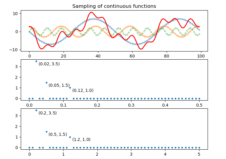
Routine 8.4: sampling of continuous functions
    # 8.4: sampling of continuous functions

    # Define a function to calculate the frequency of all basis vectors
    def gen_freq(N, fs):
        k = np.arange(0, np.floor(N/2) + 1, 1)
        return (k * fs) / N

    T = 100
    # Define multiple fundamental frequency signals with different frequencies
    fk = [2/T, 5/T, 12/T]  # frequency
    A = [7, 3, 2]  # amplitude
    phi = [np.pi, 2, 2*np.pi]  # Initial phase

    n = np.arange(T)
    s0 = A[0] * np.sin(2 * np.pi * fk[0] * n + phi[0])
    s1 = A[1] * np.sin(2 * np.pi * fk[1] * n + phi[1])
    s2 = A[2] * np.sin(2 * np.pi * fk[2] * n + phi[2])
    s = s0 + s1 + s2  # Superimpose to generate mixed signal
    g = np.fft.rfft(s)  # Fourier transform

    plt.figure(figsize=(8, 6))
    plt.subplot(311)
    plt.plot(n, s0, n, s1, n, s2, ':', marker='+', alpha=0.5)
    plt.plot(n, s, 'r-', lw=2)
    plt.title("Sampling of continuous functions")

    plt.subplot(312)
    fs = 1  # The sampling interval is 1
    freq = gen_freq(T, fs=fs)  # Calculate frequency sequence
    ck = np.abs(g) / T  # Calculate amplitude
    plt.plot(freq, ck, '.')  # Frequency amplitude diagram
    for f in fk:
        ck0 = round(ck[np.where(freq==f*fs)][0], 1)
        plt.annotate('$({},{})$'.format(f*fs, ck0), xy=(f*fs, ck0), xytext=(5, -10), textcoords='offset points')

    plt.subplot(313)
    fs = 10  # The sampling interval is 10
    freq = gen_freq(T, fs=fs)  # Calculate frequency sequence
    ck = np.abs(g) / T  # Calculate amplitude
    plt.plot(freq, ck, '.')  # Frequency amplitude diagram
    for f in fk:
        ck0 = round(ck[np.where(freq==f*fs)][0], 1)
        plt.annotate('$({},{})$'.format(f*fs, ck0), xy=(f*fs, ck0), xytext=(5, -10), textcoords='offset points')

    plt.show()
1.3 one dimensional discrete Fourier transform
Both digital signal and digital image are discrete variables obtained by sampling.
Data after sampling the transformation of the original function
F ~ ( μ ) = ∫ − ∞ + ∞ f ~ ( t ) e − j 2 π μ t d t = ∫ − ∞ + ∞ ∑ n = − ∞ ∞ f ( t ) δ ( t − n Δ T ) e − j 2 π μ t d t = ∑ n = − ∞ ∞ ∫ − ∞ + ∞ f ( t ) δ ( t − n Δ T ) e − j 2 π μ t d t = ∑ n = − ∞ ∞ f n e − j 2 π μ n Δ T \begin{aligned} \tilde{F}(\mu) &= \int_{-\infty}^{+\infty} \tilde{f}(t) e^{-j 2 \pi \mu t} dt\\ &= \int_{-\infty}^{+\infty} \sum_{n=-\infty}^{\infty} f(t) \delta (t-n{\Delta T}) e^{-j 2 \pi \mu t} dt\\ &= \sum_{n=-\infty}^{\infty} \int_{-\infty}^{+\infty} f(t) \delta (t-n{\Delta T}) e^{-j 2 \pi \mu t} dt\\ &= \sum_{n=-\infty}^{\infty} f_n e^{-j 2 \pi \mu n{\Delta T}}\\ \end{aligned} F~(μ)=∫−∞+∞f~(t)e−j2πμtdt=∫−∞+∞n=−∞∑∞f(t)δ(t−nΔT)e−j2πμtdt=n=−∞∑∞∫−∞+∞f(t)δ(t−nΔT)e−j2πμtdt=n=−∞∑∞fne−j2πμnΔT
When the sampling frequency is μ = m / M Δ T \mu = m/M \Delta T μ= m/M Δ When T, the discrete Fourier transform (DFT) and inverse transform formula can be obtained as follows:
F m = ∑ n = 0 M − 1 f n e − j 2 π μ m n / M , m = 0 , . . . M − 1 f n = 1 M ∑ m = 0 M − 1 F m e j 2 π μ m n / M , n = 0 , . . . M − 1 \begin{aligned} F_m &= \sum_{n=0}^{M-1} f_n e^{-j\ 2\pi \mu mn/M}, &m=0,...M-1\\ f_n &= \frac{1}{M} \sum_{m=0}^{M-1} F_m e^{j\ 2\pi \mu mn/M}, &n=0,...M-1 \end{aligned} Fmfn=n=0∑M−1fne−j 2πμmn/M,=M1m=0∑M−1Fmej 2πμmn/M,m=0,...M−1n=0,...M−1
Because any periodic or aperiodic function can be expressed as the sum of sine function and cosine function of different frequencies, the function characteristics expressed by Fourier transform can be reconstructed by inverse Fourier transform without losing any information. This is the mathematical basis of frequency domain image processing.
Discrete Fourier transform decomposes the discrete signal into a series of discrete trigonometric function components, and each trigonometric function component has corresponding amplitude A, frequency f and phase φ \varphi φ. The original discrete signal can be obtained by superposition of all components.
In image processing, it is usually used x , y x, y x. Y represents discrete coordinate variables in spatial domain, with u , v u,v u. V represents discrete frequency domain variables. Therefore, the one-dimensional discrete Fourier transform is expressed as:
F ( u ) = ∑ x = 0 M − 1 f ( x ) e − j 2 π u x / M , u = 0 , . . . M − 1 f ( x ) = 1 M ∑ u = 0 M − 1 F ( u ) e j 2 π u x / M , x = 0 , . . . M − 1 \begin{aligned} F(u) &= \sum_{x=0}^{M-1} f(x) e^{-j\ 2\pi u x/M}, &u=0,...M-1\\ f(x) &= \frac{1}{M} \sum_{u=0}^{M-1} F(u) e^{j\ 2\pi u x/M}, &x=0,...M-1 \end{aligned} F(u)f(x)=x=0∑M−1f(x)e−j 2πux/M,=M1u=0∑M−1F(u)ej 2πux/M,u=0,...M−1x=0,...M−1
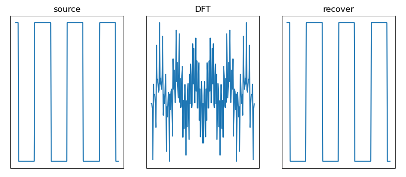
Routine 8.6: one dimensional discrete Fourier transform
    # 8.6: one dimensional discrete Fourier transform
    # Generate square wave signal
    N = 200
    t = np.linspace(-10, 10, N)
    dt = t[1] - t[0]
    sint = np.sin(t)
    sig = np.sign(sint)
    fig = plt.figure(figsize=(10, 4))
    plt.subplot(131), plt.title("source"), plt.xticks([]), plt.yticks([])
    plt.plot(t, sig)

    # Discrete Fourier transform
    fft = np.fft.fft(sig, N)  # Discrete Fourier transform
    fftshift = np.fft.fftshift(fft)  # Symmetrical translation
    amp = abs(fftshift) / len(fft)  # amplitude
    pha = np.angle(fftshift)  # phase
    fre = np.fft.fftshift(np.fft.fftfreq(d=dt, n=N))  # frequency
    plt.subplot(132), plt.title("DFT"), plt.xticks([]), plt.yticks([])
    plt.plot(t, fft)

    # Signal recovery
    recover = np.zeros(N)
    for a, p, f in zip(amp, pha, fre):
        sigCos = a * np.cos(2 * np.pi * f * np.arange(N) * dt + p)  # Construct trigonometric function according to amplitude, phase and frequency
        recover += sigCos  # Add up all these trigonometric functions

    plt.subplot(133), plt.title("recover"), plt.xticks([]), plt.yticks([])
    plt.plot(t, recover)
    plt.show()
2. Fourier transform of two-dimensional function
2.1 two dimensional continuous Fourier transform
set up f ( t , z ) f(t,z) f(t,z) is a two-dimensional continuous variable t , z t, z t. Z, then its two-dimensional continuous Fourier transform and inverse transform are:
F
(
μ
,
ν
)
=
∫
−
∞
+
∞
∫
−
∞
+
∞
f
(
t
,
z
)
e
−
j
2
π
(
μ
t
+
ν
z
)
d
t
d
z
f
(
t
,
z
)
=
∫
−
∞
+
∞
∫
−
∞
+
∞
F
(
μ
,
ν
)
e
j
2
π
(
μ
t
+
ν
z
)
d
μ
d
ν
\begin{aligned} F(\mu,\nu) &= \int_{-\infty}^{+\infty} \int_{-\infty}^{+\infty} f(t,z) e^{-j 2\pi (\mu t + \nu z)} dt \ dz\\ f(t,z) &= \int_{-\infty}^{+\infty} \int_{-\infty}^{+\infty} F(\mu,\nu) e^{j 2\pi (\mu t + \nu z)} d\mu \ d\nu \end{aligned}
F(μ,ν)f(t,z)=∫−∞+∞∫−∞+∞f(t,z)e−j2π(μt+νz)dt dz=∫−∞+∞∫−∞+∞F(μ,ν)ej2π(μt+νz)dμ dν
For image processing, the
t
,
z
t, z
t. Z represents a continuous spatial variable,
μ
,
ν
\mu, \nu
μ,ν Represents a continuous frequency variable.
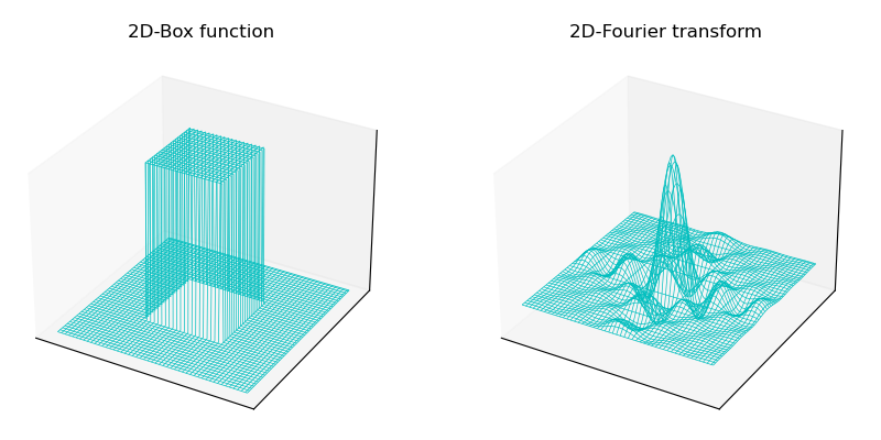
Routine 8.7: Fourier transform of two-dimensional continuous function (two-dimensional box function)
Taking the box function as an example, its Fourier transform is:
F ( μ , ν ) = ∫ − ∞ + ∞ ∫ − ∞ + ∞ f ( t , z ) e − j 2 π ( μ t + ν z ) d t d z = ∫ − T / 2 + T / 2 ∫ − Z / 2 + Z / 2 A e − j 2 π ( μ t + ν z ) d t d z = A T Z [ s i n ( π μ T ) π μ T ] [ s i n ( π ν Z ) π ν Z ] \begin{aligned} F(\mu,\nu) &= \int_{-\infty}^{+\infty} \int_{-\infty}^{+\infty} f(t,z) e^{-j 2\pi (\mu t + \nu z)} dt \ dz\\ &= \int_{-T/2}^{+T/2} \int_{-Z/2}^{+Z/2} A e^{-j 2\pi (\mu t + \nu z)} dt \ dz\\ &= ATZ[\frac{sin(\pi \mu T)}{\pi \mu T}][\frac{sin(\pi \nu Z)}{\pi \nu Z}] \end{aligned} F(μ,ν)=∫−∞+∞∫−∞+∞f(t,z)e−j2π(μt+νz)dt dz=∫−T/2+T/2∫−Z/2+Z/2Ae−j2π(μt+νz)dt dz=ATZ[πμTsin(πμT)][πνZsin(πνZ)]
    # 8.7: Fourier transform of two-dimensional continuous function (two-dimensional box function)
    # 2D box_function
    t = np.arange(-5, 5, 0.1)  # start, end, step
    z = np.arange(-5, 5, 0.1)
    height, width = len(t), len(z)
    tt, zz = np.meshgrid(t, z)  # Convert one-dimensional arrays xnew and yNew into grid point set (two-dimensional array)

    f = np.zeros([len(t), len(z)])  # Initialization, zero
    f[30:70, 30:70] = 1  # Two dimensional box function

    fu = np.sinc(t)
    fv = np.sinc(z)
    fuv = np.outer(np.sinc(t), np.sinc(z))  # Calculation of Continuous Fourier transform by formula
    print(fu.shape, fv.shape, fuv.shape)

    fig = plt.figure(figsize=(10, 6))
    ax1 = plt.subplot(121, projection='3d')
    ax1.set_title("2D-Box function")
    ax1.plot_wireframe(tt, zz, f, rstride=2, cstride=2, linewidth=0.5, color='c')
    ax1.set_xticks([]), ax1.set_yticks([]), ax1.set_zticks([])
    ax2 = plt.subplot(122, projection='3d')
    ax2.set_title("2D-Fourier transform")
    ax2.plot_wireframe(tt, zz, fuv, rstride=2, cstride=2, linewidth=0.5, color='c')
    ax2.set_xticks([]), ax2.set_yticks([]), ax2.set_zticks([])
    plt.show()
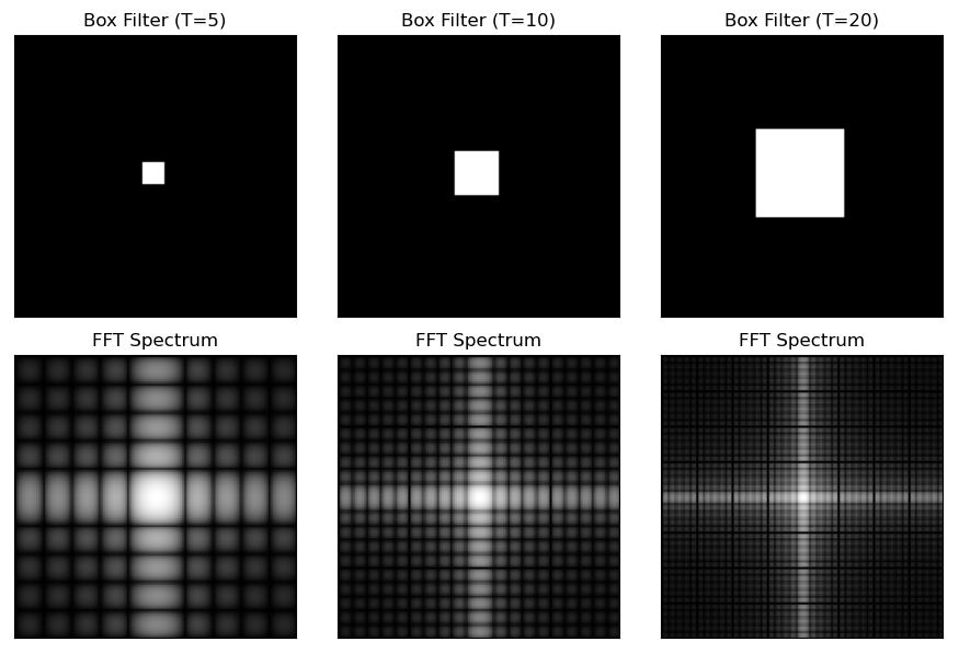
Routine 8.8: Fourier transform of two-dimensional continuous function (box function with different parameters)
    # 8.8: Fourier transform of two-dimensional continuous function (box function with different parameters)
    # 2D box_function
    height, width = 128, 128
    m = int((height - 1) / 2)
    n = int((width - 1) / 2)

    fig = plt.figure(figsize=(9, 6))
    T = [5, 10, 20]
    print(len(T))
    for i in range(len(T)):
        f = np.zeros([height, width])  # Initialization, zero
        f[m-T[i]:m+T[i], n-T[i]:n+T[i]] = 1  # Box functions of different sizes
        fft = np.fft.fft2(f)
        shift_fft = np.fft.fftshift(fft)
        amp = np.log(1 + np.abs(shift_fft))

        plt.subplot(2,len(T),i+1), plt.xticks([]), plt.yticks([])
        plt.imshow(f, "gray"), plt.title("Box Filter (T={})".format(T[i]))
        #
        plt.subplot(2,len(T),len(T)+i+1), plt.xticks([]), plt.yticks([])
        plt.imshow(amp, "gray"), plt.title("FFT Spectrum")

    plt.tight_layout()
    plt.show()
2.2 image aliasing and resampling
Since a function cannot be sampled indefinitely, aliasing always occurs in digital images.
Aliasing is divided into spatial aliasing and temporal aliasing. Spatial aliasing is caused by under sampling, which is more obvious in unfamiliar and repeated images. Time aliasing is related to the time interval of images in dynamic image sequences, such as the "wheel effect" of spoke reversal.
The main problem of spatial aliasing is the introduction of artifacts, that is, line sawtooth, false highlight and frequency mode that do not appear in the original image.
Aliasing is introduced when the image is scaled. Image enlargement can be regarded as oversampling, and the use of bilinear and bicubic interpolation can reduce the aliasing in image enlargement. Image reduction can be regarded as under sampling, and aliasing is usually more serious.
In order to reduce aliasing, a low-pass filter should be used to smooth before resampling to attenuate the high-frequency component of the image, which can effectively suppress aliasing, but the definition of the image also decreases.
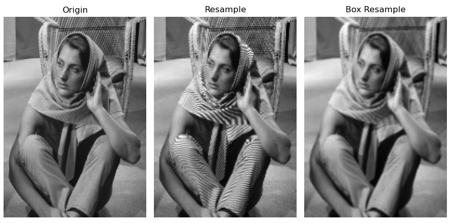
Routine 8.9: anti aliasing of images
    # 8.9: anti aliasing of images
    imgGray = cv2.imread("../images/Fig0417a.tif", flags=0)  # flags=0 read as grayscale image
    height, width = imgGray.shape[:2]  # The height and width of the picture

    # Reduce the image first and then enlarge it
    imgZoom1 = cv2.resize(imgGray, (int(0.33*width), int(0.33*height)))
    imgZoom2 = cv2.resize(imgZoom1, None, fx=3, fy=3, interpolation=cv2.INTER_AREA)

    # Firstly, 5x5 low-pass filtering is applied to the original image, then the image is reduced and then enlarged
    kSize = (5, 5)
    imgBoxFilter = cv2.boxFilter(imgGray, -1, kSize)  # cv2.boxFilter method
    imgZoom3 = cv2.resize(imgBoxFilter, (int(0.33*width), int(0.33*height)))
    imgZoom4 = cv2.resize(imgZoom3, None, fx=3, fy=3, interpolation=cv2.INTER_AREA)

    fig = plt.figure(figsize=(9,5))
    plt.subplot(131), plt.axis('off'), plt.title("Origin")
    plt.imshow(imgGray, cmap='gray')
    plt.subplot(132), plt.axis('off'), plt.title("Resample")
    plt.imshow(imgZoom2, cmap='gray')
    plt.subplot(133), plt.axis('off'), plt.title("Box Resample")
    plt.imshow(imgZoom4, cmap='gray')
    plt.tight_layout()
    plt.show()
2.3 two dimensional discrete Fourier transform (DFT)
For two-dimensional image processing, it is usually used x , y x, y x. Y represents discrete coordinate variables in spatial domain, with u , v u,v u. V represents discrete frequency domain variables. Two dimensional discrete Fourier transform (DFT) and inverse transform (IDFT) are:
F
(
u
,
v
)
=
∑
x
=
0
M
−
1
∑
y
=
0
N
−
1
f
(
x
,
y
)
e
−
j
2
π
(
u
x
/
M
+
v
y
/
N
)
f
(
x
,
y
)
=
1
M
N
∑
u
=
0
M
−
1
∑
v
=
0
N
−
1
F
(
u
,
v
)
e
j
2
π
(
u
x
/
M
+
v
y
/
N
)
\begin{aligned} F(u,v) &= \sum_{x=0}^{M-1} \sum_{y=0}^{N-1} f(x,y) e^{-j 2\pi (ux/M+vy/N)}\\ f(x,y) &= \frac{1}{MN} \sum_{u=0}^{M-1} \sum_{v=0}^{N-1} F(u,v) e^{j 2\pi (ux/M+vy/N)} \end{aligned}
F(u,v)f(x,y)=x=0∑M−1y=0∑N−1f(x,y)e−j2π(ux/M+vy/N)=MN1u=0∑M−1v=0∑N−1F(u,v)ej2π(ux/M+vy/N)
Two dimensional discrete Fourier transform can also be expressed in polar coordinates:
F
(
u
,
v
)
=
R
(
u
,
v
)
+
j
I
(
u
,
v
)
=
∣
F
(
u
,
v
)
∣
e
j
ϕ
(
u
,
v
)
F(u,v) = R(u,v) + j I(u,v) = |F(u,v)| e^{j \phi (u,v)}
F(u,v)=R(u,v)+jI(u,v)=∣F(u,v)∣ejϕ(u,v)
The Fourier spectrum is:
∣
F
(
u
,
v
)
∣
=
[
R
2
(
u
,
v
)
+
I
2
(
u
,
v
)
]
1
/
2
|F(u,v)| = [R^2(u,v) + I^2(u,v)]^{1/2}
∣F(u,v)∣=[R2(u,v)+I2(u,v)]1/2
The Fourier phase spectrum is:
ϕ
(
u
,
v
)
=
a
r
c
t
a
n
[
I
(
u
,
v
)
/
R
(
u
,
v
)
]
\phi (u,v) = arctan[I(u,v)/R(u,v)]
ϕ(u,v)=arctan[I(u,v)/R(u,v)]
The Fourier power spectrum is:
P
(
u
,
v
)
=
∣
F
(
u
,
v
)
∣
2
=
R
2
(
u
,
v
)
+
I
2
(
u
,
v
)
P(u,v) = |F(u,v)|^2 = R^2(u,v) + I^2(u,v)
P(u,v)=∣F(u,v)∣2=R2(u,v)+I2(u,v)
Spatial sampling and frequency interval correspond to each other. The interval between discrete variables corresponding to frequency domain is: Δ u = 1 / M Δ T , Δ v = 1 / N Δ Z \Delta u = 1/M \Delta T,\Delta v = 1/N \Delta Z Δ u=1/M Δ T, Δ v=1/N Δ Z. That is, the interval between samples in the frequency domain is inversely proportional to the product of the interval between spatial samples and the number of samples.
Spatial domain filter and frequency domain filter are also corresponding to each other. Two dimensional convolution theorem is the link to establish an equivalent relationship between spatial domain and frequency domain filter:
(
f
⋆
h
)
(
x
,
y
)
⇔
(
F
⋅
H
)
(
u
,
v
)
(f \star h)(x,y) \Leftrightarrow (F \cdot H)(u,v)
(f⋆h)(x,y)⇔(F⋅H)(u,v)
This shows that f and H are Fourier transforms of F and h, respectively; The Fourier transform of the spatial convolution of F and H is the product of their transformations.
Therefore, the spatial convolution of two functions can be calculated directly in the spatial domain or in the frequency domain: first calculate the Fourier transform of each function, then multiply the two transforms, and finally carry out the inverse Fourier transform to convert back to the spatial domain.
In other words, spatial domain filters and frequency domain filters are actually corresponding to each other. Some spatial domain filters will be more convenient and faster to realize by Fourier transform in frequency domain.
2.4 Numpy realizes image Fourier transform
NP in Numpy fft. FFT 2 () function can realize the Fourier transform of image.
Function Description:
numpy.fft.fft2(a, s=None, axes=(- 2, - 1), norm=None) → out
Parameter Description:
- a: Input array, one-dimensional or multi-dimensional array, can be plural
- s: The shape of the output array (the length of each transformation axis), corresponding to N in fft(x,n), optional
- out: output array, one-dimensional or multi-dimensional array in complex form (complex ndarray)
matters needing attention:
- When used for Fourier transform of two-dimensional image, the input array a is numpy two-dimensional array (gray image) or three-dimensional array (color image).
- The output is in the plural form ( R e a l + j ∗ I m a g ) (Real + j * Imag) The array of (Real+j * Imag) cannot be directly used to display images. In order to display the image of the Fourier transform result, the value of the array needs to be adjusted to the gray space of [0255].
After NP fft. The FFT 2 () function realizes the picture spectrum information obtained by Fourier transform, and the maximum value (low-frequency component) of the amplitude spectrum is at the upper left corner (0,0). For easy observation, NP is usually used fft. The fftshift() function moves the low-frequency component to the center of the frequency-domain image.
Function Description:
numpy.fft.fftshift(x, axes=None) → y
Parameter Description:
- x: Input array, one-dimensional or multi-dimensional array
- axes: integer, or tuple of input array shape. It is used to specify the axis of movement. Optional
- y: Output array
Routine 8.10: discrete Fourier transform (Numpy) of two-dimensional image
    # 8.10: Numpy realizes two-dimensional discrete Fourier transform
    normalize = lambda x: (x - x.min()) / (x.max() - x.min() + 1e-6)
    imgGray = cv2.imread("../images/Fig0424a.tif", flags=0)  # flags=0 read as grayscale image
    # imgGray = cv2.imread("../images/imgBall.png", flags=1)  # flags=0 read as grayscale image

    # Fourier transform
    # fft = np.fft.fft2(imgGray.astype(np.float32))
    fft = np.fft.fft2(imgGray)  # np. fft. Implementation of Fourier transform with FFT 2

    # Decentralize and calculate the amplitude spectrum and phase spectrum
    ampSpectrum = np.sqrt(np.power(fft.real, 2) + np.power(fft.imag, 2))  # Amplitude spectrum
    print("ampSpectrum max={}, min={}".format(ampSpectrum.max(), ampSpectrum.min()))
    # phase = np.arctan2(fft.imag, fft.real)  # Phase angle calculation (radian)
    # phiSpectrum = phase / np.pi*180  # Convert phase angle to [- 180, 180]
    phiSpectrum = np.angle(fft)

    # Centralization, moving the low-frequency component to the center of the frequency domain image
    fftShift = np.fft.fftshift(fft)  # Move the low-frequency component to the center of the frequency domain image
    # Amplitude spectrum after centralization
    ampSpeShift = np.sqrt(np.power(fftShift.real, 2) + np.power(fftShift.imag, 2))
    ampShiftNorm = np.uint8(normalize(ampSpeShift)*255)  # Normalized to [0255]
    # Logarithmic transformation of amplitude spectrum
    ampSpeLog = np.log(1 + ampSpeShift)  # The amplitude spectrum is logarithmically transformed for easy display
    ampSpeLog = np.uint8(normalize(ampSpeLog)*255)  # Normalized to [0255]

    # np. fft. Implementation of inverse Fourier transform of image using ifft2
    invShift = np.fft.ifftshift(fftShift)  # Switch the low-frequency reversal back to the four corners of the image
    imgIfft = np.fft.ifft2(invShift)  # Inverse Fourier transform, the return value is a complex array
    imgRebuild = np.abs(imgIfft)  # Adjust complex array to gray space

    plt.figure(figsize=(9, 6))
    plt.subplot(231), plt.title("Original image"), plt.axis('off')
    plt.imshow(imgGray, cmap='gray')
    plt.subplot(232), plt.title("FFT phase spectrum"), plt.axis('off')
    plt.imshow(phiSpectrum, cmap='gray')
    plt.subplot(233), plt.title("Rebuild image with IFFT"), plt.axis('off')
    plt.imshow(imgRebuild, cmap='gray')
    plt.subplot(234), plt.title("FFT amplitude spectrum"), plt.axis('off')
    plt.imshow(ampSpectrum, cmap='gray')
    plt.subplot(235), plt.title("FFT-shift amplitude"), plt.axis('off')
    plt.imshow(ampSpeShift, cmap='gray')
    plt.subplot(236), plt.title("Log-trans of FFT amp"), plt.axis('off')
    plt.imshow(ampSpeLog, cmap='gray')
    plt.tight_layout()
    plt.show()

Procedure description:
This is also the reason why it is difficult to completely process the amplitude of the center of the SPE (FFT) in the SPE (shift) image.
2.5 OpenCV realizes image Fourier transform (cv.dft)
Use cv. In OpenCV DFT () function can also realize the Fourier transform of image, CV IDFT () function realizes the inverse Fourier transform of image.
Function Description:
	cv.dft(src[, dst[, flags[, nonzeroRows]]]) → dst
	cv.idft(src[, dst[, flags[, nonzeroRows]]]) → dst
Parameter Description:
- src: input image, single channel gray image, using NP Float32 format
- dst: output image. The image size is the same as src, and the data type is determined by flag
- flag: conversion identifier
- cv. DFT_ Invert: replace the default forward transform with one-dimensional or two-dimensional inverse transform
- cv.DFT_SCALE: scale indicator, which calculates the scaling result according to the number of elements. It is often associated with DFT_ Use with invert
- cv.DFT_ROWS: forward or reverse Fourier transform is performed on each row of the input matrix, which is often used for complex operations such as three-dimensional or high-dimensional transformation
- cv.DFT_COMPLEX_OUTPUT: forward transform the one-dimensional or two-dimensional real array. The default method is the complex array represented by two channels. The first channel is the real part and the second channel is the imaginary part
- cv.DFT_REAL_OUTPUT: inverse transformation of one-dimensional or two-dimensional complex array, and the result is usually a complex matrix with the same size
matters needing attention:
- The input image src is NP Float32 format, such as images, using NP Uint8 format must be converted to NP Float32 format.
- Default method cv DFT_ COMPLEX_ When output, the input src is NP The output dst is a two-dimensional array of two channels. The first channel dft[:,:,0] is the real part and the second channel dft[:,:,1] is the imaginary part.
- Cannot be used directly to display images. You can use cv Convert the result of Fourier transform to [0255].
- idft(src, dst, flags) is equivalent to DFT (SRC, DST, flags = dft_invert).
- OpenCV realizes Fourier transform, and the calculation speed is faster than Numpy.
Convert the identifier to CV DFT_ COMPLEX_ When output, CV The output of the DFT () function is a two-dimensional array of two channels, using cv The magnitude () function can calculate the amplitude of two-dimensional vector.
Function Description:
cv.magnitude(x, y[, magnitude]) → dst
Parameter Description:
- x: One dimensional or multi-dimensional array, which also represents the real part of complex number, floating point type
- y: A one-dimensional or multi-dimensional array, which also represents the imaginary part of a complex number. It is a floating-point type. The size of the array must be the same as x
- dst: output array. The array size and data type are the same as x. the operation formula is:
d s t ( I ) = x ( I ) 2 + y ( I ) 2 dst(I) = \sqrt{x(I)^2 + y(I)^2} dst(I)=x(I)2+y(I)2
The value range of Fourier transform and related operations may not be suitable for image display, and normalization processing is required. CV. In OpenCV Normalize() function can realize image normalization.
Function Description:
cv.normalize(src, dst[, alpha[, beta[, norm_type[, dtype[, mask]]]]]) → dst
Parameter Description:
- src: input image
- dst: output result, the same size and type as the input image
- alpha: the minimum value after normalization; optional; the default value is 0
- beta: the maximum value after normalization. Optional. The default value is 1
- norm_type: normalization type
- NORM_INF: Linf norm (maximum of absolute value)
- NORM_L1: L1 norm (sum of absolute values)
- NORM_L2: L2 norm (Euclidean distance), default type
- NORM_MINMAX: linear scaling, common type
- dtype: optional. The default value is - 1, indicating that the output matrix is the same as the input image type
- Mask: mask, optional, no mask by default
Fourier transform is needed in theory O ( M N ) 2 O(MN)^2 O(MN)2 operations, very time-consuming; Fast Fourier transform only needs O ( M N l o g ( M N ) ) O(MN log (MN)) O(MNlog(MN)) operations can be completed.
Fourier transform function CV in OpenCV DFT () can decompose the number of rows and columns into 2 p ∗ 3 q ∗ 5 r 2^p * 3^q * 5^r The matrix of 2p * 3q * 5r has the best computational performance. In order to improve the operation performance, 0 can be added to the right and lower parts of the original matrix to meet the decomposition condition. CV. In OpenCV Getoptimaldftsize() function can realize the optimal DFT size expansion of the image, which is applicable to CV DFT () and NP fft. fft2().
Function Description:
cv.getOptimalDFTSize(versize) → retval
Parameter Description:
- Versione: array size
- retval: optimal array size for DFT expansion
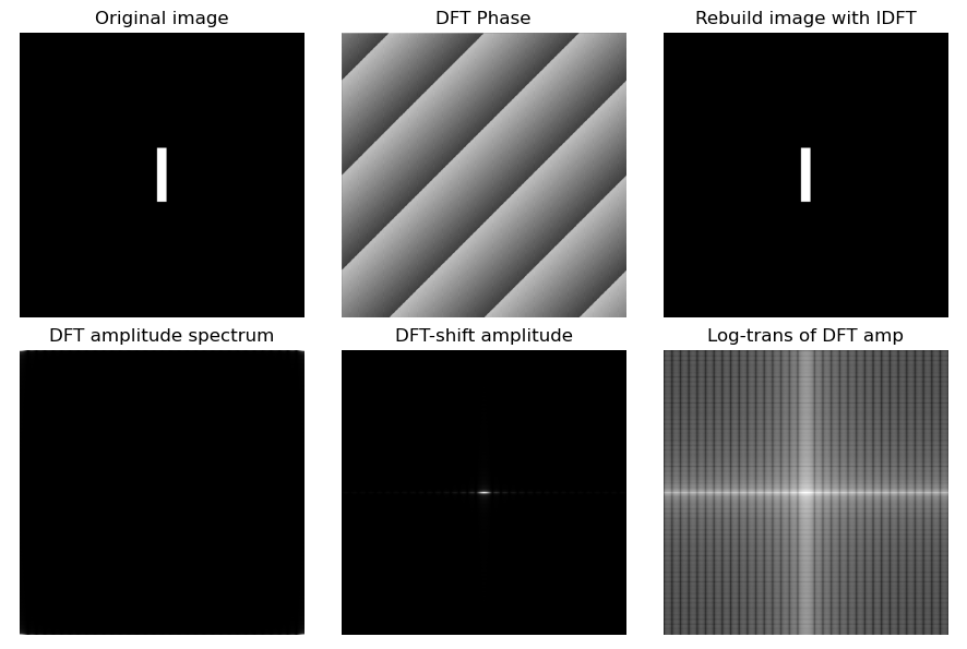
Routine 8.11: discrete Fourier transform (OpenCV) of two-dimensional image
    # 8.11: OpenCV realizes the discrete Fourier transform of two-dimensional image
    imgGray = cv2.imread("../images/Fig0424a.tif", flags=0)  # flags=0 read as grayscale image

    # cv2. Fourier transform of image based on DFT
    imgFloat32 = np.float32(imgGray)  # Convert image to float32
    dft = cv2.dft(imgFloat32, flags=cv2.DFT_COMPLEX_OUTPUT)  # Fourier transform
    dftShift = np.fft.fftshift(dft)  # Move the low-frequency component to the center of the frequency domain image

    # Amplitude spectrum
    # ampSpe = np.sqrt(np.power(dft[:,:,0], 2) + np.power(dftShift[:,:,1], 2))
    dftAmp = cv2.magnitude(dft[:,:,0], dft[:,:,1])  # Amplitude spectrum, uncentralized
    dftShiftAmp = cv2.magnitude(dftShift[:,:,0], dftShift[:,:,1])  # Amplitude spectrum, centralization
    dftAmpLog = np.log(1 + dftShiftAmp)  # Logarithmic transformation of amplitude spectrum for easy display
    # Phase spectrum
    phase = np.arctan2(dftShift[:,:,1], dftShift[:,:,0])  # Phase angle calculation (radian)
    dftPhi = phase / np.pi*180  # Convert phase angle to [- 180, 180]

    print("dftMag max={}, min={}".format(dftAmp.max(), dftAmp.min()))
    print("dftPhi max={}, min={}".format(dftPhi.max(), dftPhi.min()))
    print("dftAmpLog max={}, min={}".format(dftAmpLog.max(), dftAmpLog.min()))

    # cv2.idft implementation of image inverse Fourier transform
    invShift = np.fft.ifftshift(dftShift)  # Switch the low-frequency reversal back to the four corners of the image
    imgIdft = cv2.idft(invShift)  # Inverse Fourier transform
    imgRebuild = cv2.magnitude(imgIdft[:,:,0], imgIdft[:,:,1])  # Reconstructed image

    plt.figure(figsize=(9, 6))
    plt.subplot(231), plt.title("Original image"), plt.axis('off')
    plt.imshow(imgGray, cmap='gray')
    plt.subplot(232), plt.title("DFT Phase"), plt.axis('off')
    plt.imshow(dftPhi, cmap='gray')
    plt.subplot(233), plt.title("Rebuild image with IDFT"), plt.axis('off')
    plt.imshow(imgRebuild, cmap='gray')
    plt.subplot(234), plt.title("DFT amplitude spectrum"), plt.axis('off')
    plt.imshow(dftAmp, cmap='gray')
    plt.subplot(235), plt.title("DFT-shift amplitude"), plt.axis('off')
    plt.imshow(dftShiftAmp, cmap='gray')
    plt.subplot(236), plt.title("Log-trans of DFT amp"), plt.axis('off')
    plt.imshow(dftAmpLog, cmap='gray')
    plt.tight_layout()
    plt.show()
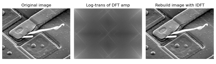
Routine 8.12: OpenCV fast Fourier transform
    # 8.12: OpenCV fast Fourier transform
    imgGray = cv2.imread("../images/Fig0429a.tif", flags=0)  # flags=0 read as grayscale image
    rows,cols = imgGray.shape[:2]  # Row (height) / column (width) of the image

    # Fast Fourier transform (matrix expansion of the original image)
    rPad = cv2.getOptimalDFTSize(rows)  # Optimal DFT expansion size
    cPad = cv2.getOptimalDFTSize(cols)  # For fast Fourier transform
    imgEx = np.zeros((rPad,cPad,2),np.float32)  # Edge expansion of the original image
    imgEx[:rows,:cols,0] = imgGray  # Edge expansion, 0 on the lower and right sides
    dftImgEx = cv2.dft(imgEx, cv2.DFT_COMPLEX_OUTPUT)  # fast Fourier transform

    # Inverse Fourier transform
    idftImg = cv2.idft(dftImgEx)  # Inverse Fourier transform
    idftMag = cv2.magnitude(idftImg[:,:,0], idftImg[:,:,1])  # Inverse Fourier transform amplitude

    # The restored image is obtained by matrix clipping
    idftMagNorm = np.uint8(cv2.normalize(idftMag, None, 0, 255, cv2.NORM_MINMAX))  # Normalized to [0255]
    imgRebuild = np.copy(idftMagNorm[:rows, :cols])

    print("max(imgGray-imgRebuild) = ", np.max(imgGray-imgRebuild))
    print("imgGray:{}, dftImg:{}, idftImg:{}, imgRebuild:{}".
          format(imgGray.shape, dftImgEx.shape, idftImg.shape, imgRebuild.shape))

    plt.figure(figsize=(9, 6))
    plt.subplot(131), plt.title("Original image"), plt.axis('off')
    plt.imshow(imgGray, cmap='gray')
    plt.subplot(132), plt.title("Log-trans of DFT amp"), plt.axis('off')
    dftAmp = cv2.magnitude(dftImgEx[:,:,0], dftImgEx[:,:,1])  # Amplitude spectrum, centralization
    dftAmpLog = np.log(1 + dftAmp)  # Logarithmic transformation of amplitude spectrum for easy display
    plt.imshow(cv2.normalize(dftAmpLog, None, 0, 255, cv2.NORM_MINMAX), cmap='gray')
    plt.subplot(133), plt.title("Rebuild image with IDFT"), plt.axis('off')
    plt.imshow(imgRebuild, cmap='gray')
    plt.tight_layout()
    plt.show()
Copyright notice:
Welcome to pay attention "Python Xiaobai OpenCV learning class from scratch @ youcans" Original works
Some of the original pictures in this article are from Rafael C. Gonzalez "Digital Image Processing, 4th.Ed." thank you.
Original works, reprint must be marked with the original link: https://blog.csdn.net/youcans/article/details/122917951
Copyright 2022 youcans, XUPT
Crated: 2022-2-14
Welcome to pay attention "100 routines" Series, continuously updating
Welcome to pay attention "Python Xiaobai's OpenCV learning course" Series, continuously updating
Python white OpenCV learning class from scratch - 1 Installation and environment configuration
Python white OpenCV learning class from scratch - 2 Image reading and display
Python white OpenCV learning class from scratch - 3 Image creation and modification
Python white OpenCV learning class from scratch - 4 Image overlay and blending
Python white OpenCV learning class from scratch - 5 Geometric transformation of image
Python white OpenCV learning class from scratch - 6 Gray transformation and histogram processing
Python white OpenCV learning class from scratch - 7 Spatial domain image filtering
Python white OpenCV learning class from scratch - 8 Frequency domain image filtering (I)