This blog will introduce three color spaces (RGB, HSV, Lab) in OpenCV and their conversion, and discuss the key role of lighting conditions and color space in computer vision applications.
The key point is to always consider lighting conditions before writing code! In general, it is easier to control lighting conditions than to write code to compensate for images captured at low quality.
- RGB color space is the most common color space in computer vision. It is simple but not intuitive, because it is difficult to accurately determine how much red, green and blue a color is composed of with the naked eye. Render as a cube.
- HSV color space is intuitive and allows colors to be defined along cylinders rather than RGB cubes. HSV color space also provides a separate dimension for brightness / whiteness, making it easier to define color depth.
- Neither RGB nor HSV can imitate the way humans perceive color, while Lab color space can perceive the difference and judge the similarity of the two colors from the Euclidean distance.
1. Renderings
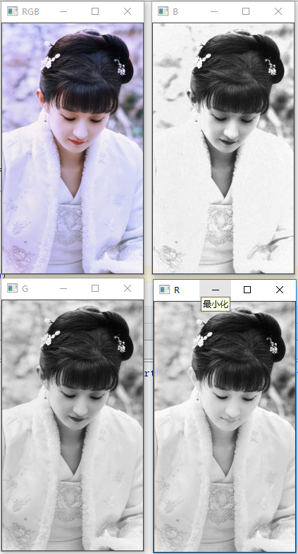
RGB original VS effect drawing of each channel is as follows:
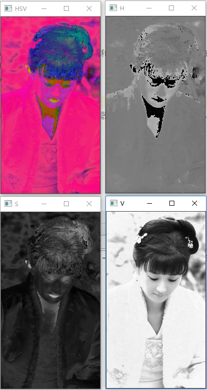
The effect drawing of HSV original VS each channel is as follows:
The Value graph is essentially a grayscale image - this is because the Value controls the actual brightness of the color, while Hue and Saturation define the actual color and shadow.
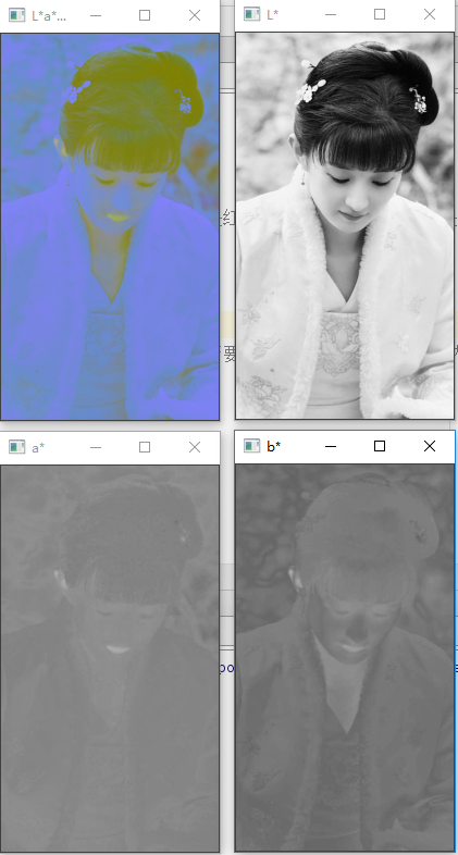
The renderings of Lab VS channels are as follows:
Similar to the HSV example, the L channel is dedicated to displaying the brightness of a given pixel. Channel A and channel b determine the shadow and color of pixels.
2. Principle
2.1 importance of lighting conditions
Lighting may mean the difference between the success and failure of computer vision algorithms. In fact, light may even be the most important factor.
Before writing code, get the ideal lighting conditions as much as possible. Controlling lighting conditions is easier than writing code to compensate for lower lighting conditions.
Three objectives should be pursued when dealing with light conditions:
-
High contrast (we should seek to maximize the contrast between regions of interest in the image (that is, the "object" that wants to detect, extract, describe, classify, operate, etc. has a sufficiently high contrast with the rest of the image, and try to ensure a high contrast between the background and foreground of the environment);
-
Scalable (lighting conditions should be consistent enough for expansion);
-
Stable (having stable, consistent and repeatable lighting conditions is the Holy Grail of computer vision application development.)
2.2 three color spaces / models in opencv
Color model is an abstract method to represent color with numbers in color space.
- RGB
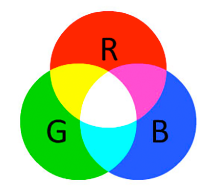
RGB represents the red, green and blue components in the image and is usually regarded as a cube.
- RGB color space is an example of additive color space: the more colors are added, the brighter the pixels are, and the closer they are to white;
- [0255] 256 values in total; Red + Green = yellow. Red + blue = pink. Red + Green + blue = white.
R=252, G=198, B=188 = white skin color.
R=22, G=159, B=230 = blue logo.
- HSV
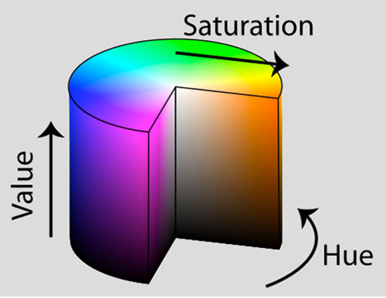
HSV color space reshapes it as a cylinder instead of a cube, and brightness is a separate dimension
- Hue: hue, which "pure" color are you checking. For example, all shadows and hues of the red color will have the same hue. [0, 179]
- Saturation: saturation, how "white" the color is. A fully saturated color will be a "solid color", such as "pure red". The color with zero saturation will be pure white. [0, 255]
- Value: allows you to control the brightness of the color. A value of zero indicates pure black, while increasing the value produces a lighter color. [0, 255]
- Lab
In RGB and HSV color space, Euclidean distance cannot "measure" the perceived difference between colors. The lab color space can imitate the human method of observing and interpreting color. Lab is a 3-axis system, which makes the Euclidean distance between two arbitrary colors have practical perceptual significance**
- L-channel: the "Brightness" of the pixel. The value varies up and down the vertical axis, from white to black, and is neutral gray at the center of the axis.
- a-channel: from the center of L channel, pure green is defined at one end of the spectrum and pure red is defined at the other end.
- Channel b: from the center of channel L, but perpendicular to channel a. b channel defines pure blue at one end and pure yellow at the other end of the spectrum. Similarly, although Lab * color space is not as intuitive and difficult to understand as HSV and RGB color space, it has been widely used in computer vision.
This is because the distance between colors has practical perceptual significance, so that we can overcome the problems of various lighting conditions. It is also used as a powerful color image descriptor.
2.3 main uses of color space
-
RGB: simple enough, mainly used to display color on the display;
-
HSV: it is easy to define a color range using HSV when you are interested in tracking objects in an image according to color.
-
Lab: it provides perceptual uniformity, which can imitate the method of human observation and interpretation of color, so that the distance between two arbitrary colors has practical significance. L * a * b color space can provide excellent color image descriptors when color management, color transmission, or color consistency across multiple devices are concerned.
-
Grayscale: it is not a color space, but in applications where the color is irrelevant, such as ignoring the color and using the grayscale representation of the image when detecting a face or building an object classifier - this can save memory and improve computational efficiency.
3. Source code
# Load images and demonstrate how to use RGB, HSV, and L*a*b * color spaces.
# USAGE
# python color_spaces.py

# Import necessary packages
import argparse
import cv2
import imutils

# Constructing command line parameters and parsing
# --Image input image path
ap = argparse.ArgumentParser()
ap.add_argument("-i", "--image", type=str, default="ml3.jpg",
                help="path to input image")
args = vars(ap.parse_args())

# Load image and display
image = cv2.imread(args["image"])
image = imutils.resize(image, width=200)
cv2.imshow("RGB", image)

# Traverse each individual channel and show
# RGB is the most commonly used color space, but it is not the most intuitive color space.
# The "white" or "Brightness" of the color is the additive combination of each red, green, and blue component.
for (name, chan) in zip(("B", "G", "R"), cv2.split(image)):
    cv2.imshow(name, chan)

# Wait for the key to close all windows
cv2.waitKey(0)
cv2.destroyAllWindows()

# HSV color space converts RGB color space and reshapes it into a cylinder instead of a cube. Brightness is a separate dimension
# -Hue: hue, which "pure" color are you checking. For example, all shadows and hues of the red color will have the same hue. [0, 179]
# -Saturation: saturation, how "white" the color is. A fully saturated color will be a "solid color", such as "pure red". The color with zero saturation will be pure white. [0, 255]
# -Value: allows you to control the brightness of the color. A value of zero indicates pure black, while increasing the value produces a lighter color. [0, 255]
# Convert the image to HSV color space and display it
hsv = cv2.cvtColor(image, cv2.COLOR_BGR2HSV)
cv2.imshow("HSV", hsv)

# Traverse each individual H, S, V channel and display
for (name, chan) in zip(("H", "S", "V"), cv2.split(hsv)):
    cv2.imshow(name, chan)

# Press to close all windows
cv2.waitKey(0)
cv2.destroyAllWindows()

# L * a * b color space
# Calculate the Euclidean distance between red and green; Red and purple; And red and navy in RGB color space:
import math

red_green = math.sqrt(((255 - 0) ** 2) + ((0 - 255) ** 2) + ((0 - 0) ** 2))
red_purple = math.sqrt(((255 - 128) ** 2) + ((0 - 0) ** 2) + ((0 - 128) ** 2))
red_navy = math.sqrt(((255 - 0) ** 2) + ((0 - 0) ** 2) + ((0 - 128) ** 2))
print(red_green, red_purple, red_navy)

# Calculating the Euclidean distance in RGB and HSV color space can not conclude that red is more similar to purple than green in a sense?,
# Euclidean distance cannot "measure" the perceived difference between colors in RGB and HSV color space.
# This is where L*a*b * color space comes into play - its goal is to imitate the way humans observe and interpret color.
# The Euclidean distance between two arbitrary colors in L*a*b * color space has practical perceptual significance.
# The addition of perceptual meaning makes L*a*b * color space less intuitive and understandable than RGB and HSV, but it is widely used in computer vision. In essence, L*a*b * color space is a 3-axis system:

# -L-channel: the "Brightness" of the pixel. The value varies up and down the vertical axis, from white to black, and is neutral gray at the center of the axis.
# -a-channel: from the center of L channel, pure green is defined at one end of the spectrum and pure red is defined at the other end.
# -Channel b: also from the center of channel L, but perpendicular to channel a. b channel defines pure blue at one end and pure yellow at the other end of the spectrum.
# Similarly, although L*a*b * color space is not as intuitive and difficult to understand as HSV and RGB color space, it has been widely used in computer vision.
# This is because the distance between colors has practical perceptual significance, so that we can overcome the problems of various lighting conditions. It is also used as a powerful color image descriptor.
# Convert the image into L*a*b space and display it
lab = cv2.cvtColor(image, cv2.COLOR_BGR2LAB)
cv2.imshow("L*a*b*", lab)
# Traverse each channel and show
for (name, chan) in zip(("L*", "a*", "b*"), cv2.split(lab)):
    cv2.imshow(name, chan)

# Wait for the key to close all windows
cv2.waitKey(0)
cv2.destroyAllWindows()

# Show grayscale image, grayscale image is not a color space
# In view of the sensitivity of the eye to color, the receptors and cones of the eye are different, so it can perceive green and red better than blue. The amount of perceived green is nearly 2 times that of red, and the amount of perceived red is more than twice that of blue,
# Therefore, when converted to gray, the weight of each RGB channel is uneven,
# Y = 0.299 \times R + 0.587 \times G + 0.114 \times B
# When the color is irrelevant, the gray representation of the image is usually used (for example, when detecting a face or building an object classifier, the color of the object is irrelevant). Therefore, discarding colors can save memory and improve computational efficiency.
gray = cv2.cvtColor(image, cv2.COLOR_BGR2GRAY)
cv2.imshow("Original", image)
cv2.imshow("Grayscale", gray)
cv2.waitKey(0)