1, Digital image processing

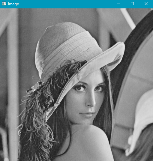
1.1 converting color image files to grayscale files

• gray image Gray image is an image with only one sampling color per pixel. This kind of image is usually displayed as a gray scale from the darkest black to the brightest white. In theory, this sampling can be different in the depth of any color, or even different colors in different brightness. gray image is different from black-and-white image. In the field of computer image, black-and-white image has only black and white Two colors; However, grayscale images have many levels of color depth between black and white. Gray level images are often obtained by measuring the brightness of each pixel in a single electromagnetic wave spectrum such as visible light. The gray level images used for display are usually saved with a nonlinear scale of 8 bits per sampling pixel, so that there can be 256 gray levels (65536 if 16 bits are used).

Using Opencv

import cv2 as cv


image = cv.imread('lena.png')
gray_image = cv.cvtColor(image, code=cv.COLOR_BGR2GRAY)

# display picture
cv.imshow('image', gray_image)
cv.waitKey(0)
cv.destroyAllWindows()

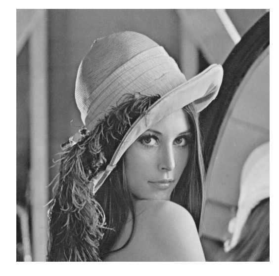
Do not use Opencv

rom PIL import Image
Img = Image.open('lena.png')
Img.show()
Le = Img.convert('L')
Le.show()

1.2 convert color images (RGB) to HSV and HSI formats

Introduction to image format

1. RGB model

3D coordinates:

The central axis from the origin to the white vertex is a gray line. The three components r, g and b are equal, and the intensity can be expressed by the vector of the three components.

Use RGB to understand the changes of color, depth and light and shade:

Color change: the connecting line between the RGB maximum component vertex of the three coordinate axes and the yellow purple green YMC color vertex

Depth variation: the distance from RGB and CMY vertices to the central axis of the origin and white vertices

Light and shade change: the position of the point of the central axis is darker at the origin and brighter at the white vertex.

2. HSV model

Inverted cone model:

This model is described by color, depth and light and shade.

H is color

S is the depth, and when S = 0, there is only gray scale

V is light and shade, indicating the brightness of the color, but it has no direct relationship with the light intensity.

3.HSI model

Hue: refers to the color attribute of a solid color (hue is related to wavelength, which is people's perception of different colors);
Saturation: a measure of the degree to which a solid color is diluted by white light (the greater the saturation, the brighter the color);
Intensity: it is a subjective factor, which is actually immeasurable (brightness and image gray are the brightness of color).
Generally speaking, H = hue; Decide what color it is, S = saturation (purity); decide the color intensity, B = brightness (brightness); decide how bright the white light shines on the color. This explanation is a real answer I've seen to understand what HSI is.

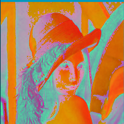
• To HSV

mport cv2 as cv
image = cv.imread('Lena.png')
hsv = cv.cvtColor(image, cv.COLOR_BGR2HSV)
# display picture
cv.imshow('hsv',hsv)
# Wait for keyboard input
cv.waitKey(0)

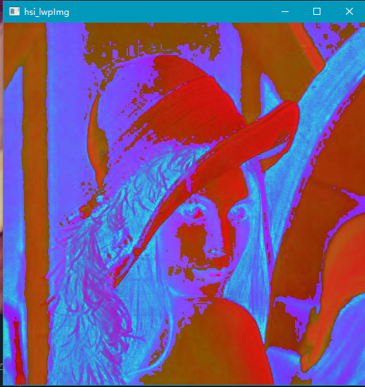
• Transfer to HSI

import cv2
import numpy as np

def rgbtohsi(rgb_lwpImg):
  rows = int(rgb_lwpImg.shape[0])
  cols = int(rgb_lwpImg.shape[1])
  b, g, r = cv2.split(rgb_lwpImg)
  # Normalized to [0,1]
  b = b / 255.0
  g = g / 255.0
  r = r / 255.0
  hsi_lwpImg = rgb_lwpImg.copy()
  H, S, I = cv2.split(hsi_lwpImg)
  for i in range(rows):
    for j in range(cols):
      num = 0.5 * ((r[i, j]-g[i, j])+(r[i, j]-b[i, j]))
      den = np.sqrt((r[i, j]-g[i, j])**2+(r[i, j]-b[i, j])*(g[i, j]-b[i, j]))
      theta = float(np.arccos(num/den))

      if den == 0:
          H = 0
      elif b[i, j] <= g[i, j]:
        H = theta
      else:
        H = 2*3.14169265 - theta

      min_RGB = min(min(b[i, j], g[i, j]), r[i, j])
      sum = b[i, j]+g[i, j]+r[i, j]
      if sum == 0:
        S = 0
      else:
        S = 1 - 3*min_RGB/sum

      H = H/(2*3.14159265)
      I = sum/3.0
      # The HSI image is output and expanded to 255 to facilitate display. Generally, the H component is between [0,2pi], and the S and I are between [0,1]
      hsi_lwpImg[i, j, 0] = H*255
      hsi_lwpImg[i, j, 1] = S*255
      hsi_lwpImg[i, j, 2] = I*255
  return hsi_lwpImg


if __name__ == '__main__':
  rgb_lwpImg = cv2.imread("lena.png")
  hsi_lwpImg = rgbtohsi(rgb_lwpImg)
  cv2.imshow('hsi_lwpImg', hsi_lwpImg)

  key = cv2.waitKey(0) & 0xFF
  if key == ord('q'):
    cv2.destroyAllWindows()

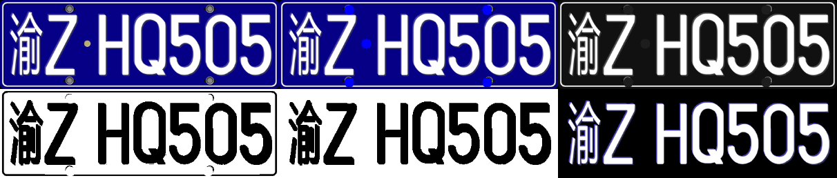
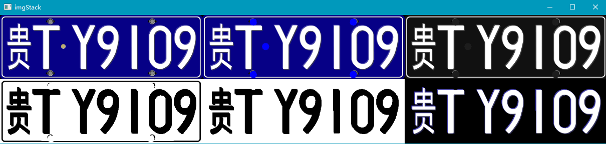
2, Split license plate

Firstly, the license plate number image is grayed out, then the pixel threshold at 5% is calculated, and finally the grayscale image is binarized.
Remove the interference surrounded by white borders around the license plate number, and then segment the characters according to the vertical projection width and accumulated values of the license plate picture.

Using Opencv

• code

import cv2
import numpy as np
import os
def stackImages(scale, imgArray):
    """
        Press multiple images into the same window for display
        :param scale:float Type, output image display percentage, control zoom scale, 0.5=The image resolution is reduced by half
        :param imgArray:Tuple nested list, image matrix to be arranged
        :return:Output image
    """
    rows = len(imgArray)
    cols = len(imgArray[0])

    rowsAvailable = isinstance(imgArray[0], list)

    # Fill in with empty pictures
    for i in range(rows):
        tmp = cols - len(imgArray[i])
        for j in range(tmp):
            img = np.zeros((imgArray[0][0].shape[0], imgArray[0][0].shape[1]), dtype='uint8')
            imgArray[i].append(img)

    # Judgment dimension
    if rows>=2:
        width = imgArray[0][0].shape[1]
        height = imgArray[0][0].shape[0]

    else:
        width = imgArray[0].shape[1]
        height = imgArray[0].shape[0]

    if rowsAvailable:
        for x in range(0, rows):
            for y in range(0, cols):
                if imgArray[x][y].shape[:2] == imgArray[0][0].shape[:2]:
                    imgArray[x][y] = cv2.resize(imgArray[x][y], (0, 0), None, scale, scale)
                else:
                    imgArray[x][y] = cv2.resize(imgArray[x][y], (imgArray[0][0].shape[1], imgArray[0][0].shape[0]),
                                                None, scale, scale)
                if len(imgArray[x][y].shape) == 2:
                    imgArray[x][y] = cv2.cvtColor(imgArray[x][y], cv2.COLOR_GRAY2BGR)
        imageBlank = np.zeros((height, width, 3), np.uint8)
        hor = [imageBlank] * rows
        hor_con = [imageBlank] * rows
        for x in range(0, rows):
            hor[x] = np.hstack(imgArray[x])
        ver = np.vstack(hor)
    else:
        for x in range(0, rows):
            if imgArray[x].shape[:2] == imgArray[0].shape[:2]:
                imgArray[x] = cv2.resize(imgArray[x], (0, 0), None, scale, scale)
            else:
                imgArray[x] = cv2.resize(imgArray[x], (imgArray[0].shape[1], imgArray[0].shape[0]), None, scale, scale)
            if len(imgArray[x].shape) == 2: imgArray[x] = cv2.cvtColor(imgArray[x], cv2.COLOR_GRAY2BGR)
        hor = np.hstack(imgArray)
        ver = hor
    return ver
# Segmentation result output path
output_dir = "D:\\MyworkSpace\\Spyder\\bmp\\pint\\"
# License plate path
file_path="D:\\MyworkSpace\\Spyder\\bmp\\pin\\"
# Read all license plates
cars = os.listdir(file_path)
cars.sort()

# Cycle each license plate
for car in cars:
    # Read picture
    print("Processing"+file_path+car)
    src = cv2.imread(file_path+car)
    img = src.copy()

    # Pretreatment to remove screw points
    cv2.circle(img, (145, 20), 10, (255, 0, 0), thickness=-1)
    cv2.circle(img, (430, 20), 10, (255, 0, 0), thickness=-1)
    cv2.circle(img, (145, 170), 10, (255, 0, 0), thickness=-1)
    cv2.circle(img, (430, 170), 10, (255, 0, 0), thickness=-1)
    cv2.circle(img, (180, 90), 10, (255, 0, 0), thickness=-1)

    # Turn gray
    gray = cv2.cvtColor(img, cv2.COLOR_BGR2GRAY)

    # Binarization
    adaptive_thresh = cv2.adaptiveThreshold(gray, 255, cv2.ADAPTIVE_THRESH_MEAN_C, cv2.THRESH_BINARY_INV, 333, 1)

    # Closed operation
    kernel = np.ones((5, 5), int)
    morphologyEx = cv2.morphologyEx(adaptive_thresh, cv2.MORPH_CLOSE, kernel)

    # Find boundary
    contours, hierarchy = cv2.findContours(morphologyEx, cv2.RETR_LIST, cv2.CHAIN_APPROX_SIMPLE)

    # Draw boundary
    img_1 = img.copy()
    cv2.drawContours(img_1, contours, -1, (0, 0, 0), -1)

    imgStack = stackImages(0.7, ([src, img, gray], [adaptive_thresh, morphologyEx, img_1]))
    cv2.imshow("imgStack", imgStack)
    cv2.waitKey(0)

    # Turn gray to facilitate cutting
    gray_1 = cv2.cvtColor(img_1, cv2.COLOR_BGR2GRAY)

    # Number of white in each column
    white = []
    # Number of black in each column
    black = []
    # The area height depends on the image height
    height = gray_1.shape[0]
    # The area width depends on the width of the picture
    width = gray_1.shape[1]
    # Maximum white quantity
    white_max = 0
    # Maximum number of black
    black_max = 0
    # Calculate the sum of black and white pixels for each column
    for i in range(width):
        s = 0  # The total number of white in this column
        t = 0  # Total number of black in this column
        for j in range(height):
            if gray_1[j][i] == 255:
                s += 1
            if gray_1[j][i] == 0:
                t += 1
        white_max = max(white_max, s)
        black_max = max(black_max, t)
        white.append(s)
        black.append(t)


    # Right boundary found
    def find_end(start):
        end = start + 1
        for m in range(start + 1, width - 1):
            # Basically all black columns are treated as boundaries
            if black[m] >= black_max * 0.95:  # Please adjust the parameter of 0.95 more, corresponding to 0.05 below
                end = m
                break
        return end


    # Temporary variable
    n = 1

    # Starting position
    start = 1

    # End position
    end = 2

    # Number of segmentation results
    num=0

    # Segmentation results
    res = []

    # Save the segmentation result path and name it with the picture name
    output_path= output_dir + car.split('.')[0]
    if not os.path.exists(output_path):
        os.makedirs(output_path)
    # Traverse from left to right
    while n < width - 2:
        n += 1

        # Find white to determine the starting address
        # You cannot directly white [n] > white_ max
        if white[n] > 0.05 * white_max:
            start = n
            # Find end coordinates
            end = find_end(start)
            # Start address of next
            n = end

            # Make sure what you find meets the requirements. It's too small, not the license plate number
            if end - start > 10:
                # division
                char = gray_1[1:height, start - 5:end + 5]
                # Save split results to file
                cv2.imwrite(output_path+'/' + str(num) + '.jpg',char)
                num+=1
                # Redraw size
                char = cv2.resize(char, (300, 300), interpolation=cv2.INTER_CUBIC)
                # Add to result collection
                res.append(char)

                # cv2.imshow("imgStack", char)
                # cv2.waitKey(0)

    # The result of the construction is convenient for the display of the result of Yuanzu
    res2 = (res[:2], res[2:4], res[4:6], res[6:])
    # Display results
    imgStack = stackImages(0.5, res2)
    cv2.imshow("imgStack", imgStack)
    cv2.waitKey(0)

• The image is grayed and binarized
  

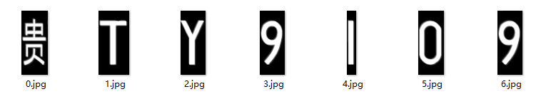
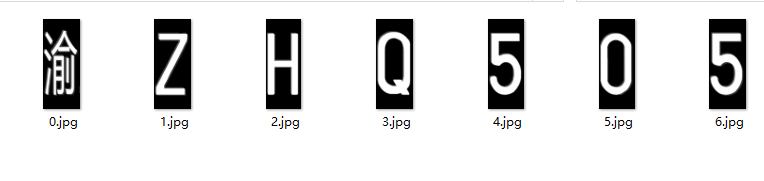
• Segmentation results
  
  

summary

• In the use of OpenCV ready-made package, the image processing will be much simpler. After being familiar with the basic principle of OpenCV, it is more convenient to process image processing.