youcans OpenCV learning course - 8 Frequency domain image filtering (Part 2)
This series is for Python Xiaobai and explains the actual combat of OpenCV project from scratch.
Image filtering is a common image preprocessing operation to suppress the noise of the target image while preserving the detailed features of the image as much as possible.
Frequency domain image processing first carries out the Fourier transform of the image, then processes it in the transform domain, and finally carries out the inverse Fourier transform to transform it back to the spatial domain.
Frequency domain filtering is the multiplication of the filter transfer function and the corresponding pixel of the Fourier transform of the input image. The concept of filtering in frequency domain is more intuitive and the filter design is easier. Using fast Fourier transform algorithm is much faster than spatial convolution.
This paper provides the complete routines and running results of the above algorithms, and demonstrates the comprehensive use of a variety of image enhancement methods through an application case.
Welcome to pay attention "OpenCV learning course of youcans" Series, continuously updated
3. Low pass filter in frequency domain
Image transformation is the transformation of image information to maintain but redistribute energy, so as to filter noise and strengthen the parts or features of interest.
3.1 fundamentals of image filtering in frequency domain
The purpose of Fourier transform is to transform the image from spatial domain to frequency domain, and realize the processing of specific information in the image in the frequency domain. It has important applications in image analysis, image enhancement, image denoising, edge detection, feature extraction, image compression and encryption.
Spatial sampling and frequency interval correspond to each other. The interval between samples in the frequency domain is inversely proportional to the product of the interval between spatial samples and the number of samples.
The spatial domain filter and the frequency domain filter also correspond to each other, and they form a Fourier transform pair:
f
(
x
,
y
)
⊗
h
(
x
,
y
)
⇔
F
(
u
,
v
)
H
(
u
,
v
)
f
(
x
,
y
)
h
(
x
,
y
)
⇔
F
(
u
,
v
)
⊗
H
(
u
,
v
)
f(x,y) \otimes h(x,y) \Leftrightarrow F(u,v)H(u,v) \\f(x,y) h(x,y) \Leftrightarrow F(u,v) \otimes H(u,v)
f(x,y)⊗h(x,y)⇔F(u,v)H(u,v)f(x,y)h(x,y)⇔F(u,v)⊗H(u,v)
In other words, spatial domain filters and frequency domain filters are actually corresponding to each other. Some spatial domain filters will be more convenient and faster to realize by Fourier transform in frequency domain.
After the Fourier transform of the signal or image, the low-frequency information and high-frequency information of the signal or image can be obtained. The low-frequency information corresponds to the slowly changing gray-scale component in the image, and the high-frequency information corresponds to the sharply changing gray-scale component.
Low pass filtering is to retain the low-frequency information of Fourier transform and weaken the high-frequency information, while high pass filtering is to retain the high-frequency information of Fourier transform and weaken the low-frequency information.
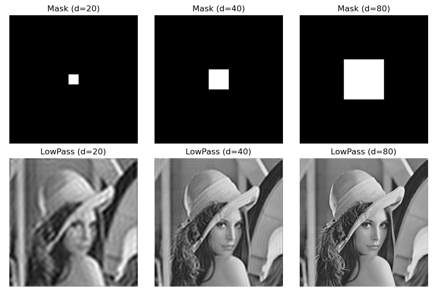
The closer it is to the center of the filter, the closer it is to the center of the filter, and the closer it is to the center of the low-frequency structure, the closer it is to the center of the filter. Simply, a rectangular window mask is generated, and a white (Set 1) window is opened in the center of the black (set 0) mask image to obtain a low-pass filter.
Routine 8.13: simple frequency domain image filtering
    # 8.13: simple frequency domain image filtering (window mask low-pass filter)
    imgGray = cv2.imread("../images/imgLena.tif", flags=0)  # flags=0 read as grayscale image
    height, width = imgGray.shape[:2]  # The height and width of the picture
    centerY, centerX = int(height/2), int(width/2)  # Picture center

    # (1) First, Fourier transform the image
    imgFloat32 = np.float32(imgGray)  # Convert image to float32
    dft = cv2.dft(imgFloat32, flags=cv2.DFT_COMPLEX_OUTPUT)  # Fourier transform
    dftShift = np.fft.fftshift(dft)  # Move the low-frequency component to the center of the frequency domain image

    d = [20, 40, 80]
    plt.figure(figsize=(9, 6))
    for i in range(3):
        # Construct a rectangular window mask for low-pass filter
        mask = np.zeros((height, width, 2), np.uint8)
        mask[centerY-d[i]:centerY+d[i], centerX-d[i]:centerX+d[i]] = 1  # Set low-pass filter rectangular window mask to filter high frequency
        maskAmp = np.uint8(np.sqrt(np.power(mask[:,:,0], 2) + np.power(mask[:,:,1], 2)))
        print("d={}, maskAmp: max={}, min={}".format(d[i],maskAmp.max(), maskAmp.min()))

        # (2) Then modify the Fourier transform in the frequency domain
        dftMask = dftShift * mask  # Modified Fourier transform to realize filtering

        # (3) Finally, the inverse Fourier transform is used to return to the spatial domain
        iShift = np.fft.ifftshift(dftMask)  # Switch the low-frequency reversal back to the four corners of the image
        iDft = cv2.idft(iShift)  # Inverse Fourier transform
        imgRebuild = cv2.magnitude(iDft[:,:,0], iDft[:,:,1])  # Reconstructed image

        plt.subplot(2,3,i+1), plt.title("Mask (d={})".format(d[i])), plt.axis('off')
        plt.imshow(maskAmp, cmap='gray')
        plt.subplot(2,3,i+4), plt.title("LowPass (d={})".format(d[i])), plt.axis('off')
        plt.imshow(imgRebuild, cmap='gray')

    plt.tight_layout()
    plt.show()
Procedure description:
This routine constructs rectangular window masks of different sizes. The center low frequency is set to 1 (white) and the surrounding high frequency is set to 0 (black). It is a low-pass filter.
The low-pass filter mask is multiplied by the image Fourier transform dftShift to make the high-frequency part of the Fourier transform 0, so as to shield the high-frequency signal in the original image and realize low-pass filtering.
Similarly, reversing the low-pass filter rectangular window mask in this routine to set the center high frequency to 0 (black) and the surrounding low frequency to 1 (white) is a high pass filter, which can realize image sharpening and edge extraction.
3.2 steps of image filtering in frequency domain
In the previous routine, a simple low-pass filter mask is multiplied by the image Fourier transform dftShift to make the high-frequency part of the Fourier transform 0, so as to shield the high-frequency signal in the original image and realize low-pass filtering.
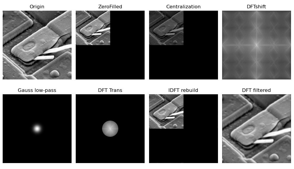
First, the original image is filtered in frequency domain f ( x , y ) f(x,y) f(x,y) is transformed into F ( u , v ) F(u,v) F(u,v), and then use the appropriate filter function H ( u , v ) H(u,v) H(u,v) pair Fourier transform F ( u , v ) F(u,v) The spectral components of F(u,v) are modified, and finally the enhanced image is obtained by returning to the spatial domain through inverse Fourier transform (IDFT) g ( x , y ) g(x,y) g(x,y).
f ( x , y ) → D F T F ( u , v ) → filter wave H ( u , v ) G ( u , v ) → I D F T g ( x , y ) f(x,y) \xrightarrow {DFT} F(u,v) \xrightarrow [filter] {H(u,v)} G(u,v) \xrightarrow {IDFT} g(x,y) f(x,y)DFT F(u,v)H(u,v) Filtering G(u,v)IDFT g(x,y)
The basic steps of image filtering in frequency domain are as follows:
(1) On the original image
f
(
x
,
y
)
f(x,y)
f(x,y) is Fourier transformed to obtain
F
(
u
,
v
)
F(u,v)
F(u,v);
(2) Fourier transform of image
F
(
u
,
v
)
F(u,v)
F(u,v) and transfer function
H
(
u
,
v
)
H(u,v)
H(u,v) is convoluted to obtain the filtered spectrum
G
(
u
,
v
)
G(u,v)
G(u,v);
(3) Right
G
(
u
,
v
)
G(u,v)
G(u,v) carries out inverse Fourier transform to obtain the enhanced image
g
(
x
,
y
)
g(x,y)
g(x,y).
Centralization is to shift the frequency spectrum to the origin. The centralized image spectrum is symmetrically distributed with the origin as the center. Moving the frequency spectrum to the center of the circle can not only clearly see the image frequency distribution, but also separate the periodic interference signals.
Routine 8.15: general steps of image filtering in frequency domain
    # # 8.15: general steps of image filtering in frequency domain (this example corresponds to figure 4.35 of P183 in the fourth edition of Gonzalez Digital Image Processing)
    imgGray = cv2.imread("../images/Fig0431.tif", flags=0)  # flags=0 read as grayscale image
    H, W = imgGray.shape[:2]  # Height (H) and width (W) of the picture
    P, Q = 2*H, 2*W
    # centerY, centerX = int(H/2), int(W/2)  # Picture center
    fig = plt.figure(figsize=(10, 6))

    # Here, the original image is pad to get better display
    imgDouble = np.ones([2*H, 2*W]) * 255
    imgDouble[:H, W:] = imgGray # The original image is on the upper right
    plt.subplot(241), plt.axis('off'), plt.title("Origin")
    # plt.imshow(imgDouble, cmap='gray')
    plt.imshow(imgGray, cmap='gray')

    fp = np.pad(imgGray, ((0,H), (0,W)), mode='constant')  # Zero fill
    plt.subplot(242), plt.axis('off'), plt.title("ZeroFilled")
    plt.imshow(fp, cmap='gray')

    # Centralization
    mask = np.ones(fp.shape)
    mask[1::2, ::2] = -1
    mask[::2, 1::2] = -1
    fpCen = fp * mask
    fpCenShow = np.clip(fpCen, 0, 255)  # Truncation function, limiting the value to [0255]
    print("fpCenShow.shape", fpCenShow.shape, fpCenShow.min(), fpCenShow.max())
    plt.subplot(243), plt.axis('off'), plt.title("Centralization")
    plt.imshow(fpCenShow, cmap='gray')

    # cv2. Fourier transform of image based on DFT
    imgFloat32 = np.float32(fp)  # Convert image to float32
    dft = cv2.dft(imgFloat32, flags=cv2.DFT_COMPLEX_OUTPUT)  # Fourier transform
    dftShift = np.fft.fftshift(dft)  # Move the low-frequency component to the center of the frequency domain image
    dftShiftAmp = cv2.magnitude(dftShift[:,:,0], dftShift[:,:,1])  # Amplitude spectrum, centralization
    dftAmpLog = np.log(1 + dftShiftAmp)  # Logarithmic transformation of amplitude spectrum for easy display
    plt.subplot(244), plt.axis('off'), plt.title("DFTshift")
    plt.imshow(dftAmpLog, cmap='gray')

    # Gauss low_pass filter: 1/(2*pi*s2) * exp(-(x**2+y**2)/(2*s2))
    sigma2 = 0.005  # square of sigma
    x, y = np.mgrid[-1:1:1.0/H, -1:1:1.0/W]
    z = 1 / (2 * np.pi * sigma2) * np.exp(-(x**2 + y**2) / (2*sigma2))
    # maskGauss = np.uint8(255 * (z - z.min()) / (z.max() - z.min()))
    maskGauss = np.uint8(cv2.normalize(z, None, 0, 255, cv2.NORM_MINMAX))  # Normalized to [0255]
    print("maskGauss.shape", maskGauss.shape, maskGauss.min(), maskGauss.max())
    plt.subplot(245), plt.axis('off'), plt.title("Gauss low-pass")
    plt.imshow(maskGauss, cmap='gray')

    maskGauss2 = np.zeros((maskGauss.shape[0], maskGauss.shape[1], 2), np.uint8)
    maskGauss2[:, :, 0] = maskGauss
    maskGauss2[:, :, 1] = maskGauss
    dftTrans = dftShift * maskGauss2  # Modified Fourier transform to realize filtering
    dftTransAmp = cv2.magnitude(dftTrans[:,:,0], dftTrans[:,:,1])  # Amplitude, centration, spectrum
    dftTransLog = np.log(1 + dftTransAmp)  # Logarithmic transformation of amplitude spectrum for easy display
    plt.subplot(246), plt.axis('off'), plt.title("DFT Trans")
    plt.imshow(dftTransLog, cmap='gray')

    # Return to spatial domain through inverse Fourier transform
    ishift = np.fft.ifftshift(dftTrans)  # Switch the low-frequency reversal back to the four corners of the image
    idft = cv2.idft(ishift)  # Inverse Fourier transform
    idftMag = cv2.magnitude(idft[:,:,0], idft[:,:,1])  # Reconstructed image
    plt.subplot(247), plt.axis('off'), plt.title("IDFT rebuild")
    plt.imshow(idftMag, cmap='gray')

    imgRebuild = idftMag[:H, :W]
    plt.subplot(248), plt.axis('off'), plt.title("DFT filtered")
    plt.imshow(imgRebuild, cmap='gray')

    plt.tight_layout()
    plt.show()
Routine 8.16: general steps of image filtering in frequency domain (ideal low-pass filter)
    # 8.16: general steps of image filtering in frequency domain (this example corresponds to the Python implementation of P383 low-pass filtering refined by Zhang Ping OpenCV algorithm)
    # (1) Read original image
    # imgGray = cv2.imread("../images/imgLena.tif", flags=0)  # flags=0 read as grayscale image
    imgGray = cv2.imread("../images/Fig0431.tif", flags=0)  # flags=0 read as grayscale image
    imgFloat32 = np.float32(imgGray)  # Convert image to float32
    rows, cols = imgGray.shape[:2]  # The height and width of the picture

    fig = plt.figure(figsize=(10, 6))
    plt.subplot(241), plt.axis('off'), plt.title("Origin image")
    plt.imshow(imgGray, cmap='gray')

    # (2) Centralized 2D array f (x, y) * - 1 ^ (x + y)
    mask = np.ones(imgGray.shape)
    mask[1::2, ::2] = -1
    mask[::2, 1::2] = -1
    fImage = imgFloat32 * mask  # f(x,y) * (-1)^(x+y)
    plt.subplot(242), plt.axis('off'), plt.title("f(x,y)*(-1)^(x+y)")
    plt.imshow(fImage, cmap='gray')

    # (3) Fast Fourier transform
    rPadded = cv2.getOptimalDFTSize(rows)  # Optimal DFT expansion size
    cPadded = cv2.getOptimalDFTSize(cols)  # For fast Fourier transform
    dftImage = np.zeros((rPadded, cPadded, 2), np.float32)  # Edge expansion of the original image
    dftImage[:rows, :cols, 0] = fImage  # Edge expansion, 0 on the lower and right sides
    cv2.dft(dftImage, dftImage, cv2.DFT_COMPLEX_OUTPUT)  # fast Fourier transform

    dftAmp = cv2.magnitude(dftImage[:,:,0], dftImage[:,:,1])  # Amplitude spectrum of Fourier transform (rPad, cPad)
    dftAmpLog = np.log(1.0 + dftAmp)  # Logarithmic transformation of amplitude spectrum for easy display
    dftAmpNorm = np.uint8(cv2.normalize(dftAmpLog, None, 0, 255, cv2.NORM_MINMAX))  # Normalized to [0255]
    plt.subplot(243), plt.axis('off'), plt.title("DFT spectrum")
    plt.imshow(dftAmpNorm, cmap='gray')

    # (4) Construction of low pass filter transfer function
    # Find the location of the maximum Fourier spectrum
    minValue, maxValue, minLoc, maxLoc = cv2.minMaxLoc(dftAmp)
    rPadded, cPadded = dftImage.shape[:2]  # Fast Fourier transform size, original image size optimization
    u, v = np.mgrid[0:rPadded:1, 0:cPadded:1]
    Dsquare = np.power((u-maxLoc[1]), 2.0) + np.power((v-maxLoc[0]), 2.0)
    D0 = 50  # radius
    D = np.sqrt(Dsquare)
    lpFilter = np.zeros(dftImage.shape[:2], np.float32)
    lpFilter[D <= D0] = 1  # Ideal low pass filter
    plt.subplot(244), plt.axis('off'), plt.title("LP Filter")
    plt.imshow(lpFilter, cmap='gray')

    # (5) Modify Fourier transform in frequency domain: Fourier transform point multiplication low-pass filter
    # rPadded, cPadded = dftImage.shape[:2]  # Fast Fourier transform size, original image size optimization
    dftLPfilter = np.zeros(dftImage.shape, dftImage.dtype)  # Size of fast Fourier transform (optimized size)
    for i in range(2):
        dftLPfilter[:rPadded, :cPadded, i] = dftImage[:rPadded, :cPadded, i] * lpFilter

    # Fourier spectrum of low-pass Fourier transform
    lpDftAmp = cv2.magnitude(dftLPfilter[:, :, 0], dftLPfilter[:, :, 1])  # Amplitude spectrum of Fourier transform
    lpDftAmpLog = np.log(1.0 + lpDftAmp)  # Logarithmic transformation of amplitude spectrum for easy display
    lpDftAmpNorm = np.uint8(cv2.normalize(lpDftAmpLog, None, 0, 255, cv2.NORM_MINMAX))  # Normalized to [0255]
    plt.subplot(245), plt.axis('off'), plt.title("lpfDft Spectrum")
    plt.imshow(lpDftAmpNorm, cmap='gray')

    # (6) The inverse Fourier transform is performed on the low-pass Fourier transform, and only the real part is taken
    idft = np.zeros(dftAmp.shape, np.float32)  # Size of fast Fourier transform (optimized size)
    cv2.dft(dftLPfilter, idft, cv2.DFT_REAL_OUTPUT + cv2.DFT_INVERSE + cv2.DFT_SCALE)
    plt.subplot(246), plt.axis('off'), plt.title("IDFT Spectrum")
    plt.imshow(idft, cmap='gray')

    # (7) Centralized 2D array g (x, y) * - 1 ^ (x + y)
    mask2 = np.ones(dftAmp.shape)
    mask2[1::2, ::2] = -1
    mask2[::2, 1::2] = -1
    idftCen = idft * mask2  # g(x,y) * (-1)^(x+y)
    plt.subplot(247), plt.axis('off'), plt.title("g(x,y)*(-1)^(x+y)")
    plt.imshow(idftCen, cmap='gray')

    # (8) Intercept the upper left corner, the size is equal to the input image
    result = np.clip(idftCen, 0, 255)  # Truncation function, limiting the value to [0255]
    lpResult = result.astype(np.uint8)
    lpResult = lpResult[:rows, :cols]

    plt.subplot(248), plt.axis('off'), plt.title("DFT filtered")
    plt.imshow(lpResult, cmap='gray')
    plt.tight_layout()
    plt.show()

    print("image.shape:{}".format(imgGray.shape))
    print("imgFloat32.shape:{}".format(imgFloat32.shape))
    print("dftImage.shape:{}".format(dftImage.shape))
    print("dftAmp.shape:{}".format(dftAmp.shape))
    print("idft.shape:{}".format(idft.shape))
    print("lpFilter.shape:{}".format(lpFilter.shape))
    print("result.shape:{}".format(result.shape))
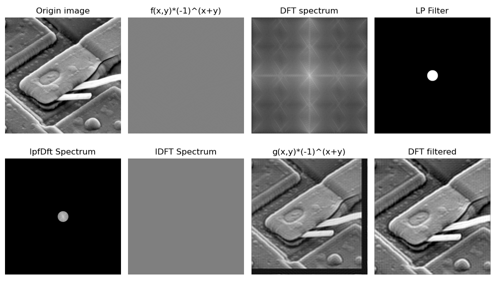
Procedure description:
(1) Use CV2 Getoptimaldftsize() obtains the optimized size of the fast Fourier transform and performs edge expansion and 0 filling on the original image, so it is not necessarily the same as the original image. After frequency domain filtering, the upper left corner is intercepted to obtain a filtered image with the same size as the original image.
(2) Note that the size of the filter should be the same as that of the (fast) Fourier transform, not necessarily the same as that of the original image.
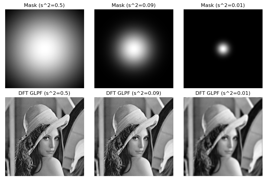
3.3 frequency domain Gaussian low pass filter (GLPF)
Routine 8.16 takes the ideal low-pass filter as an example and gives the general steps of image filtering in frequency domain.
The filtering effect of Gaussian filter changes with the distance from the sample point to the center of Fourier transform. When the distance increases, the filtering effect becomes better.
The frequency domain Gaussian low-pass filter is also a mask:
H
(
u
,
v
)
=
e
−
(
u
2
+
v
2
)
/
2
σ
2
D
(
u
,
v
)
=
(
u
−
P
/
2
)
2
+
(
v
−
Q
/
2
)
2
H(u,v) = e^{-(u^2+v^2)/2 \sigma^2}\\ D(u,v) = \sqrt {(u-P/2)^2+(v-Q/2)^2}
H(u,v)=e−(u2+v2)/2σ2D(u,v)=(u−P/2)2+(v−Q/2)2
Where
D
0
=
σ
D_0=\sigma
D0= σ Is the cut-off frequency when
D
(
u
,
v
)
=
D
0
D(u,v) = D_0
When D(u,v)=D0, GLPF decreases to 0.607 of the maximum value.
Using two-dimensional Gaussian mask, high frequency can be filtered out and low frequency can be retained. Variance of Gaussian function in frequency domain σ 2 \sigma^2 σ The smaller the Gaussian function is, the narrower the Gaussian function is, the more high-frequency components (image details) are filtered, and the more blurred the image is.
The amount of computation of Gaussian filter in spatial domain increases with the increase of template, while the amount of computation of Gaussian filter in frequency domain is independent of filter function.
Routine 8.18: frequency domain Gaussian low pass filter (GLPF)
    # 8.18: frequency domain Gaussian low pass filter (GLPF)
    imgGray = cv2.imread("../images/imgLena.tif", flags=0)  # flags=0 read as grayscale image

    # (1) First, Fourier transform the image
    imgFloat32 = np.float32(imgGray)  # Convert image to float32
    dft = cv2.dft(imgFloat32, flags=cv2.DFT_COMPLEX_OUTPUT)  # Fourier transform
    dftShift = np.fft.fftshift(dft)  # Move the low-frequency component to the center of the frequency domain image

    # # Amplitude spectrum
    # imgDFT = 10 * np.log(cv2.magnitude(dftShift[:,:,0], dftShift[:,:,1]))
    # plt.figure(figsize=(9, 6))
    # plt.subplot(121), plt.axis('off'), plt.title("Original"), plt.imshow(imgGray, 'gray')
    # plt.subplot(122), plt.axis('off'), plt.title("FFt"), plt.imshow(imgDFT, cmap='gray')
    # plt.show()

    plt.figure(figsize=(9, 6))
    rows, cols = imgGray.shape[:2]  # The height and width of the picture
    sigma2 = [0.5, 0.09, 0.01]  # square of sigma
    for i in range(3):
        # Construct Gaussian filter mask:# Gauss = 1/(2*pi*s2) * exp(-(x**2+y**2)/(2*s2))
        x, y = np.mgrid[-1:1:2.0 / rows, -1:1:2.0 / cols]
        z = 1 / (2 * np.pi * sigma2[i]) * np.exp(-(x ** 2 + y ** 2) / (2 * sigma2[i]))
        # maskGauss = np.uint8(cv2.normalize(z, None, 0, 255, cv2.NORM_MINMAX))  # Normalized to [0255]
        zNorm = np.uint8(cv2.normalize(z, None, 0, 255, cv2.NORM_MINMAX))  # Normalized to [0255]
        maskGauss = np.zeros((rows, cols, 2), np.uint8)
        maskGauss[:,:,0] = zNorm
        maskGauss[:,:,1] = zNorm
        print(maskGauss.shape, maskGauss.max(), maskGauss.min())

        # (2) Then modify the Fourier transform in the frequency domain
        dftTrans = dftShift * maskGauss  # Modified Fourier transform to realize filtering

        # (3) Finally, the inverse Fourier transform is used to return to the spatial domain
        ishift = np.fft.ifftshift(dftTrans)  # Switch the low-frequency reversal back to the four corners of the image
        idft = cv2.idft(ishift)  # Inverse Fourier transform
        imgRebuild = cv2.magnitude(idft[:,:,0], idft[:,:,1])  # Reconstructed image

        plt.subplot(2,3,i+1), plt.title("Mask (s^2={})".format(sigma2[i])), plt.axis('off')
        plt.imshow(maskGauss[:,:,0], cmap='gray')
        plt.subplot(2,3,i+4), plt.title("DFT GLPF (s^2={})".format(sigma2[i])), plt.axis('off')
        plt.imshow(imgRebuild, cmap='gray')

    plt.tight_layout()
    plt.show()
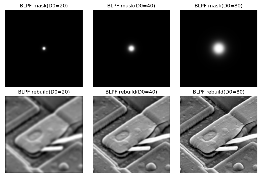
3.4 frequency domain Butterworth low pass filter (BLPF)
The cut-off frequency is located at the center of the frequency
D
0
D_0
The transfer function of the n-order Butterworth low-pass filter at D0 ¢ is:
H
(
u
,
v
)
=
1
1
+
[
D
(
u
,
v
)
/
D
0
]
2
n
H(u,v) = \frac {1}{1+[D(u,v) / D_0]^{2n}}
H(u,v)=1+[D(u,v)/D0]2n1
When n is large, Butterworth low-pass filter BLPF can approach the characteristics of ideal low-pass filter ILPF; When n is small, Butterworth low-pass filter BLPF can approximate the characteristics of Gaussian low-pass filter GLPF and provide a smooth transition from low frequency to high frequency.
Using two-dimensional Gaussian mask, high frequency can be filtered out and low frequency can be retained. The smaller the frequency domain Gaussian function is, the narrower the Gaussian function is, the more high-frequency components (image details) are filtered, and the more blurred the image is.
The characteristic of Butterworth filter is that the frequency response curve in the pass band is flat to the greatest extent without fluctuation, while it gradually drops to zero in the stop band.
On the Bode diagram of logarithmic diagonal frequency of amplitude, starting from the boundary angular frequency of one side, the amplitude gradually decreases with the increase of angular frequency and tends to negative infinity. The frequency characteristic curve of Butterworth filter is a monotonic function of frequency in both passband and stopband. Therefore, when the boundary of the passband meets the index requirements, there will be margin in the passband. Therefore, a more effective design method should be to evenly distribute the accuracy in the whole passband or stopband, or both.
Routine 8.19: frequency domain Butterworth low pass filter (BLPF)
    # 8.19: frequency domain Butterworth low pass filter (BLPF)
    # (1) Read original image
    # imgGray = cv2.imread("../images/imgLena.tif", flags=0)  # flags=0 read as grayscale image
    imgGray = cv2.imread("../images/Fig0431.tif", flags=0)  # flags=0 read as grayscale image
    imgFloat32 = np.float32(imgGray)  # Convert image to float32
    rows, cols = imgGray.shape[:2]  # The height and width of the picture

    # (2) Centralized 2D array f (x, y) * - 1 ^ (x + y)
    mask = np.ones(imgGray.shape)
    mask[1::2, ::2] = -1
    mask[::2, 1::2] = -1
    fImage = imgFloat32 * mask  # f(x,y) * (-1)^(x+y)

    # (3) Fast Fourier transform
    # dftImage = fft2Image(fImage)  # Fast Fourier transform (rPad, cPad, 2)
    rPadded = cv2.getOptimalDFTSize(rows)  # Optimal DFT expansion size
    cPadded = cv2.getOptimalDFTSize(cols)  # For fast Fourier transform
    dftImage = np.zeros((rPadded, cPadded, 2), np.float32)  # Edge expansion of the original image
    dftImage[:rows, :cols, 0] = fImage  # Edge expansion, 0 on the lower and right sides
    cv2.dft(dftImage, dftImage, cv2.DFT_COMPLEX_OUTPUT)  # fast Fourier transform

    dftAmp = cv2.magnitude(dftImage[:,:,0], dftImage[:,:,1])  # Amplitude spectrum of Fourier transform (rPad, cPad)
    dftAmpLog = np.log(1.0 + dftAmp)  # Logarithmic transformation of amplitude spectrum for easy display
    dftAmpNorm = np.uint8(cv2.normalize(dftAmpLog, None, 0, 255, cv2.NORM_MINMAX))  # Normalized to [0255]
    minValue, maxValue, minLoc, maxLoc = cv2.minMaxLoc(dftAmp)  # Find the location of the maximum Fourier spectrum

    plt.figure(figsize=(9, 6))
    # rows, cols = imgGray.shape[:2]  # The height and width of the picture
    u, v = np.mgrid[0:rPadded:1, 0:cPadded:1]
    D = np.sqrt(np.power((u-maxLoc[1]), 2) + np.power((v-maxLoc[0]), 2))
    D0 = [20, 40, 80]  # cut-off frequency
    n = 2
    for k in range(3):
        # (4) Construction of low pass filter transfer function
        # Butterworth low pass filter
        epsilon = 1e-8  # Prevent division by 0
        lpFilter = 1.0 / (1.0 + np.power(D / (D0[k] + epsilon), 2*n))

        # (5) Modify Fourier transform in frequency domain: Fourier transform point multiplication low-pass filter
        dftLPfilter = np.zeros(dftImage.shape, dftImage.dtype)  # Size of fast Fourier transform (optimized size)
        for j in range(2):
            dftLPfilter[:rPadded, :cPadded, j] = dftImage[:rPadded, :cPadded, j] * lpFilter

        # (6) The inverse Fourier transform is performed on the low-pass Fourier transform, and only the real part is taken
        idft = np.zeros(dftAmp.shape, np.float32)  # Size of fast Fourier transform (optimized size)
        cv2.dft(dftLPfilter, idft, cv2.DFT_REAL_OUTPUT + cv2.DFT_INVERSE + cv2.DFT_SCALE)

        # (7) Centralized 2D array g (x, y) * - 1 ^ (x + y)
        mask2 = np.ones(dftAmp.shape)
        mask2[1::2, ::2] = -1
        mask2[::2, 1::2] = -1
        idftCen = idft * mask2  # g(x,y) * (-1)^(x+y)

        # (8) Intercept the upper left corner, the size is equal to the input image
        result = np.clip(idftCen, 0, 255)  # Truncation function, limiting the value to [0255]
        imgBLPF = result.astype(np.uint8)
        imgBLPF = imgBLPF[:rows, :cols]

        plt.subplot(2,3,k+1), plt.title("BLPF mask(D0={})".format(D0[k])), plt.axis('off')
        plt.imshow(lpFilter[:,:], cmap='gray')
        plt.subplot(2,3,k+4), plt.title("BLPF rebuild(D0={})".format(D0[k])), plt.axis('off')
        plt.imshow(imgBLPF, cmap='gray')

    plt.tight_layout()
    plt.show()
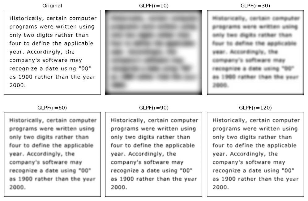
3.5 low pass filtering case in frequency domain: character restoration of printed text
Low pass filtering technology is mainly used in printing and publishing industry. This section presents the practical application of low-pass filtering in frequency domain: character restoration of printed text. The case comes from figure 4.48 of P194 of Gonzalez's digital image processing (Fourth Edition).
The original image is a sample of a low resolution text image. We will encounter such text in fax, copy or historical documents. The text in the picture does not have stains, creases and tears, but the characters in the text are distorted due to insufficient resolution, many of which are broken. One way to solve this problem is to bridge these small gaps by blurring the input image.
The routine shows how to use different D 0 D_0 The repair effect of D0 # Gaussian low-pass filter after simple processing. Of course, this is only one step of repair. Next, other processing, such as threshold processing and thinning processing, will be carried out. These methods will be discussed in the follow-up content.
In order to facilitate future use, the routine encapsulates the optimal extended fast Fourier transform and Gaussian low-pass filter as functions.
    # 8.22: GLPF low-pass filtering case: text character recognition
    def gaussLowPassFilter(shape, radius=10):  # Gaussian low pass filter
        # Gaussian filter:# Gauss = 1/(2*pi*s2) * exp(-(x**2+y**2)/(2*s2))
        u, v = np.mgrid[-1:1:2.0/shape[0], -1:1:2.0/shape[1]]
        D = np.sqrt(u**2 + v**2)
        D0 = radius / shape[0]
        kernel = np.exp(- (D ** 2) / (2 *D0**2))
        return kernel

    def dft2Image(image):  #Optimal extended fast Fourier transform
        # Centralized 2D array f (x, y) * - 1 ^ (x + y)
        mask = np.ones(image.shape)
        mask[1::2, ::2] = -1
        mask[::2, 1::2] = -1
        fImage = image * mask  # f(x,y) * (-1)^(x+y)

        # Optimal DFT expansion size
        rows, cols = image.shape[:2]  # The height and width of the original picture
        rPadded = cv2.getOptimalDFTSize(rows)  # Optimal DFT expansion size
        cPadded = cv2.getOptimalDFTSize(cols)  # For fast Fourier transform

        # Edge extension (complement 0), fast Fourier transform
        dftImage = np.zeros((rPadded, cPadded, 2), np.float32)  # Edge expansion of the original image
        dftImage[:rows, :cols, 0] = fImage  # Edge expansion, 0 on the lower and right sides
        cv2.dft(dftImage, dftImage, cv2.DFT_COMPLEX_OUTPUT)  # fast Fourier transform
        return dftImage


    # (1) Read original image
    imgGray = cv2.imread("../images/Fig0419a.tif", flags=0)  # flags=0 read as grayscale image
    rows, cols = imgGray.shape[:2]  # The height and width of the picture

    plt.figure(figsize=(10, 6))
    plt.subplot(2, 3, 1), plt.title("Original"), plt.axis('off'), plt.imshow(imgGray, cmap='gray')

    # (2) Fast Fourier transform
    dftImage = dft2Image(imgGray)  # Fast Fourier transform (rPad, cPad, 2)
    rPadded, cPadded = dftImage.shape[:2]  # Fast Fourier transform size, original image size optimization
    print("dftImage.shape:{}".format(dftImage.shape))


    D0 = [10, 30, 60, 90, 120]  # radius
    for k in range(5):
        # (3) Construct Gaussian low pass filter
        lpFilter = gaussLowPassFilter((rPadded, cPadded), radius=D0[k])

        # (5) Modify Fourier transform in frequency domain: Fourier transform point multiplication low-pass filter
        dftLPfilter = np.zeros(dftImage.shape, dftImage.dtype)  # Size of fast Fourier transform (optimized size)
        for j in range(2):
            dftLPfilter[:rPadded, :cPadded, j] = dftImage[:rPadded, :cPadded, j] * lpFilter

        # (6) The inverse Fourier transform is performed on the low-pass Fourier transform, and only the real part is taken
        idft = np.zeros(dftImage.shape[:2], np.float32)  # Size of fast Fourier transform (optimized size)
        cv2.dft(dftLPfilter, idft, cv2.DFT_REAL_OUTPUT + cv2.DFT_INVERSE + cv2.DFT_SCALE)

        # (7) Centralized 2D array g (x, y) * - 1 ^ (x + y)
        mask2 = np.ones(dftImage.shape[:2])
        mask2[1::2, ::2] = -1
        mask2[::2, 1::2] = -1
        idftCen = idft * mask2  # g(x,y) * (-1)^(x+y)

        # (8) Intercept the upper left corner, the size is equal to the input image
        result = np.clip(idftCen, 0, 255)  # Truncation function, limiting the value to [0255]
        imgLPF = result.astype(np.uint8)
        imgLPF = imgLPF[:rows, :cols]

        plt.subplot(2,3,k+2), plt.title("GLPF rebuild(n={})".format(D0[k])), plt.axis('off')
        plt.imshow(imgLPF, cmap='gray')

    print("image.shape:{}".format(imgGray.shape))
    print("lpFilter.shape:{}".format(lpFilter.shape))
    print("dftImage.shape:{}".format(dftImage.shape))

    plt.tight_layout()
    plt.show()
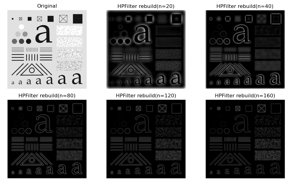
4. High pass filter in frequency domain
Image edge and other sharp changes of gray level are related to high-frequency components, so image sharpening can be realized by high pass filtering in frequency domain. High pass filtering attenuates the low-frequency components in the Fourier transform without interfering with the high-frequency information.
4.1 get high pass filter from low pass filter
Simply, by subtracting the transfer function of the low-pass filter from 1 in the frequency domain, the corresponding high-pass filter transfer function can be obtained:
H
H
P
(
u
,
v
)
=
1
−
H
L
P
(
u
,
v
)
H_{HP}(u,v) = 1- H_{LP}(u,v)
HHP(u,v)=1−HLP(u,v)
Where,
H
H
P
(
u
,
v
)
H_{HP}(u,v)
HHP(u,v),
H
L
P
(
u
,
v
)
H_{LP}(u,v)
HLP (u,v) represents the transfer functions of high pass filter and low-pass filter respectively.
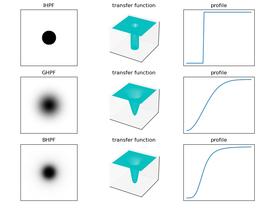
The transfer function of the ideal high pass filter (IHPF) is:
H
(
u
,
v
)
=
{
0
,
D
(
u
,
v
)
≤
D
0
1
,
D
(
u
,
v
)
>
D
0
H(u,v)=\begin{cases} 0,\ D(u,v) \leq D_0\\ 1,\ D(u,v)>D_0 \end{cases}
H(u,v)={0, D(u,v)≤D01, D(u,v)>D0
The transfer function of Gaussian high pass filter (GHPF) is:
H
(
u
,
v
)
=
1
−
e
−
D
2
(
u
,
v
)
/
2
D
0
2
H(u,v)=1-e^{-D^2 (u,v)/2D_0^2}
H(u,v)=1−e−D2(u,v)/2D02
The transfer function of Butterworth high pass filter (BHPF) is:
H
(
u
,
v
)
=
1
1
+
[
D
0
/
D
(
u
,
v
)
]
2
n
H(u,v)= \frac {1} {1 + [D_0/D(u,v)]^{2n}}
H(u,v)=1+[D0/D(u,v)]2n1
Routine 8.23 get high pass filter from low pass filter
    # 8.23: high pass filter in frequency domain
    def ideaHighPassFilter(shape, radius=10):  # Ideal high pass filter
        u, v = np.mgrid[-1:1:2.0/shape[0], -1:1:2.0/shape[1]]
        D = np.sqrt(u**2 + v**2)
        D0 = radius / shape[0]
        kernel = np.ones(shape)
        kernel[D <= D0] = 0  # Ideal low pass filter
        return kernel

    def gaussHighPassFilter(shape, radius=10):  # Gaussian Highpass Filter
        # Gaussian filter:# Gauss = 1/(2*pi*s2) * exp(-(x**2+y**2)/(2*s2))
        u, v = np.mgrid[-1:1:2.0/shape[0], -1:1:2.0/shape[1]]
        D = np.sqrt(u**2 + v**2)
        D0 = radius / shape[0]
        kernel = 1 - np.exp(- (D ** 2) / (2 *D0**2))
        return kernel

    def butterworthHighPassFilter(shape, radius=10, n=2):  # Butterworth high pass filter
        u, v = np.mgrid[-1:1:2.0/shape[0], -1:1:2.0/shape[1]]
        epsilon = 1e-8
        D = np.sqrt(u**2 + v**2)
        D0 = radius / shape[0]
        kernel = 1.0 / (1.0 + np.power(D0/(D + epsilon), 2*n))

        return kernel

    # Ideal, Gauss, Butterworth high pass transfer function
    shape = [128, 128]
    radius = 32
    IHPF = ideaHighPassFilter(shape, radius=radius)
    GHPF = gaussHighPassFilter(shape, radius=radius)
    BHPF = butterworthHighPassFilter(shape, radius=radius)

    filters = ['IHPF', 'GHPF', 'BHPF']
    u, v = np.mgrid[-1:1:2.0/shape[0], -1:1:2.0/shape[1]]
    fig = plt.figure(figsize=(10, 8))
    for i in range(3):
        hpFilter = eval(filters[i]).copy()

        ax1 = fig.add_subplot(3, 3, 3*i+1)
        ax1.imshow(hpFilter, 'gray')
        ax1.set_title(filters[i]), ax1.set_xticks([]), ax1.set_yticks([])

        ax2 = plt.subplot(3,3,3*i+2, projection='3d')
        ax2.set_title("transfer function")
        ax2.plot_wireframe(u, v, hpFilter , rstride=2, linewidth=0.5, color='c')
        ax2.set_xticks([]), ax2.set_yticks([]), ax2.set_zticks([])

        ax3 = plt.subplot(3,3,3*i+3)
        profile = hpFilter[shape[0]//2:, shape[1]//2]
        ax3.plot(profile), ax3.set_title("profile"), ax3.set_xticks([]), ax3.set_yticks([])

    plt.show()
Routine 8.24 application of high pass filter in frequency domain
    # 8.24: application of high pass filter in frequency domain
    def ideaHighPassFilter(shape, radius=10):  # Ideal high pass filter
        u, v = np.mgrid[-1:1:2.0/shape[0], -1:1:2.0/shape[1]]
        D = np.sqrt(u**2 + v**2)
        D0 = radius / shape[0]
        kernel = np.ones(shape)
        kernel[D <= D0] = 0  # Ideal low pass filter
        return kernel

    def gaussHighPassFilter(shape, radius=10):  # Gaussian Highpass Filter
        # Gaussian filter:# Gauss = 1/(2*pi*s2) * exp(-(x**2+y**2)/(2*s2))
        u, v = np.mgrid[-1:1:2.0/shape[0], -1:1:2.0/shape[1]]
        D = np.sqrt(u**2 + v**2)
        D0 = radius / shape[0]
        kernel = 1 - np.exp(- (D ** 2) / (2 *D0**2))
        return kernel

    def butterworthHighPassFilter(shape, radius=10, n=2):  # Butterworth high pass filter
        u, v = np.mgrid[-1:1:2.0/shape[0], -1:1:2.0/shape[1]]
        epsilon = 1e-8
        D = np.sqrt(u**2 + v**2)
        D0 = radius / shape[0]
        kernel = 1.0 / (1.0 + np.power(D0/(D + epsilon), 2*n))

        return kernel

    def dft2Image(image):  #Optimal extended fast Fourier transform
        # Centralized 2D array f (x, y) * - 1 ^ (x + y)
        mask = np.ones(image.shape)
        mask[1::2, ::2] = -1
        mask[::2, 1::2] = -1
        fImage = image * mask  # f(x,y) * (-1)^(x+y)

        # Optimal DFT expansion size
        rows, cols = image.shape[:2]  # The height and width of the original picture
        rPadded = cv2.getOptimalDFTSize(rows)  # Optimal DFT expansion size
        cPadded = cv2.getOptimalDFTSize(cols)  # For fast Fourier transform

        # Edge extension (complement 0), fast Fourier transform
        dftImage = np.zeros((rPadded, cPadded, 2), np.float32)  # Edge expansion of the original image
        dftImage[:rows, :cols, 0] = fImage  # Edge expansion, 0 on the lower and right sides
        cv2.dft(dftImage, dftImage, cv2.DFT_COMPLEX_OUTPUT)  # fast Fourier transform
        return dftImage


    # (1) Read original image
    imgGray = cv2.imread("../images/Fig0515a.tif", flags=0)  # flags=0 read as grayscale image
    # imgGray = cv2.imread("../images/imgLena.tif", flags=0)  # flags=0 read as grayscale image
    rows, cols = imgGray.shape[:2]  # The height and width of the picture

    plt.figure(figsize=(10, 6))
    plt.subplot(2, 3, 1), plt.title("Original"), plt.axis('off'), plt.imshow(imgGray, cmap='gray')

    # (2) Fast Fourier transform
    dftImage = dft2Image(imgGray)  # Fast Fourier transform (rPad, cPad, 2)
    rPadded, cPadded = dftImage.shape[:2]  # Fast Fourier transform size, original image size optimization
    print("dftImage.shape:{}".format(dftImage.shape))


    D0 = [20, 40, 80, 120, 160]  # radius
    for k in range(5):
        # (3) Construction of high pass filter
        # hpFilter = ideaHighPassFilter((rPadded, cPadded), radius=D0[k])  # Ideal high pass filter
        # hpFilter = gaussHighPassFilter((rPadded, cPadded), radius=D0[k])  # Gaussian Highpass Filter
        hpFilter = butterworthHighPassFilter((rPadded, cPadded), radius=D0[k])  # Butterworth Highpass Filters

        # (5) Modify Fourier transform in frequency domain: Fourier transform point multiplication low-pass filter
        dftHPfilter = np.zeros(dftImage.shape, dftImage.dtype)  # Size of fast Fourier transform (optimized size)
        for j in range(2):
            dftHPfilter[:rPadded, :cPadded, j] = dftImage[:rPadded, :cPadded, j] * hpFilter

        # (6) The high pass Fourier transform is performed only on the inverse part
        idft = np.zeros(dftImage.shape[:2], np.float32)  # Size of fast Fourier transform (optimized size)
        cv2.dft(dftHPfilter, idft, cv2.DFT_REAL_OUTPUT + cv2.DFT_INVERSE + cv2.DFT_SCALE)

        # (7) Centralized 2D array g (x, y) * - 1 ^ (x + y)
        mask2 = np.ones(dftImage.shape[:2])
        mask2[1::2, ::2] = -1
        mask2[::2, 1::2] = -1
        idftCen = idft * mask2  # g(x,y) * (-1)^(x+y)

        # (8) Intercept the upper left corner, the size is equal to the input image
        result = np.clip(idftCen, 0, 255)  # Truncation function, limiting the value to [0255]
        imgHPF = result.astype(np.uint8)
        imgHPF = imgLPF[:rows, :cols]

        plt.subplot(2,3,k+2), plt.title("HPFilter rebuild(n={})".format(D0[k])), plt.axis('off')
        plt.imshow(imgHPF, cmap='gray')

    print("image.shape:{}".format(imgGray.shape))
    print("hpFilter.shape:{}".format(hpFilter.shape))
    print("dftImage.shape:{}".format(dftImage.shape))

    plt.tight_layout()
    plt.show()
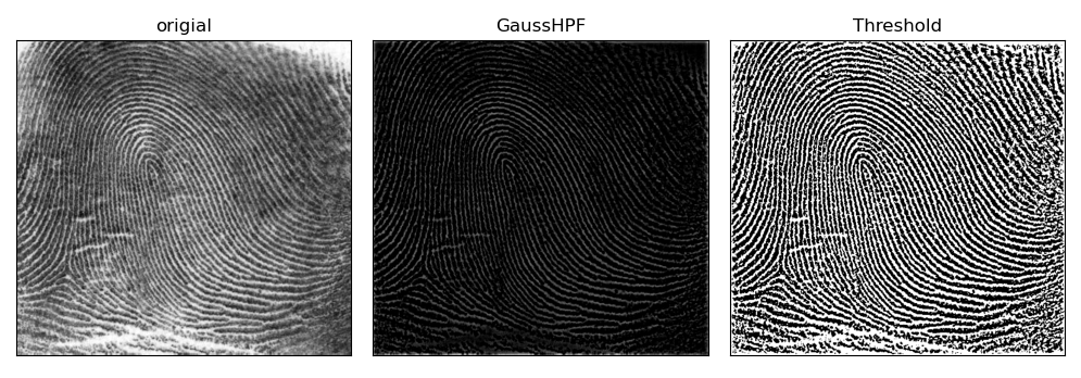
Routine 8.25: fingerprint image processing (high pass filtering + threshold processing)
    # 8.25: fingerprint image processing (high pass filtering + threshold processing)
    def gaussHighPassFilter(shape, radius=10):  # Gaussian Highpass Filter
        # Gaussian filter:# Gauss = 1/(2*pi*s2) * exp(-(x**2+y**2)/(2*s2))
        u, v = np.mgrid[-1:1:2.0/shape[0], -1:1:2.0/shape[1]]
        D = np.sqrt(u**2 + v**2)
        D0 = radius / shape[0]
        kernel = 1 - np.exp(- (D ** 2) / (2 *D0**2))
        return kernel

    def dft2Image(image):  #Optimal extended fast Fourier transform
        # Centralized 2D array f (x, y) * - 1 ^ (x + y)
        mask = np.ones(image.shape)
        mask[1::2, ::2] = -1
        mask[::2, 1::2] = -1
        fImage = image * mask  # f(x,y) * (-1)^(x+y)

        # Optimal DFT expansion size
        rows, cols = image.shape[:2]  # The height and width of the original picture
        rPadded = cv2.getOptimalDFTSize(rows)  # Optimal DFT expansion size
        cPadded = cv2.getOptimalDFTSize(cols)  # For fast Fourier transform

        # Edge extension (complement 0), fast Fourier transform
        dftImage = np.zeros((rPadded, cPadded, 2), np.float32)  # Edge expansion of the original image
        dftImage[:rows, :cols, 0] = fImage  # Edge expansion, 0 on the lower and right sides
        cv2.dft(dftImage, dftImage, cv2.DFT_COMPLEX_OUTPUT)  # fast Fourier transform
        return dftImage


    def imgHPFilter(image, D0=50):  #Image high pass filtering
        rows, cols = image.shape[:2]  # The height and width of the picture
        # fast Fourier transform
        dftImage = dft2Image(image)  # Fast Fourier transform (rPad, cPad, 2)
        rPadded, cPadded = dftImage.shape[:2]  # Fast Fourier transform size, original image size optimization

        # Construct Gaussian low pass filter
        hpFilter = gaussHighPassFilter((rPadded, cPadded), radius=D0)  # Gaussian Highpass Filter

        # Modify Fourier transform in frequency domain: Fourier transform point multiplication high pass filter
        dftHPfilter = np.zeros(dftImage.shape, dftImage.dtype)  # Size of fast Fourier transform (optimized size)
        for j in range(2):
            dftHPfilter[:rPadded, :cPadded, j] = dftImage[:rPadded, :cPadded, j] * hpFilter

        # The inverse Fourier transform is performed on the high pass Fourier transform and only the real part is taken
        idft = np.zeros(dftImage.shape[:2], np.float32)  # Size of fast Fourier transform (optimized size)
        cv2.dft(dftHPfilter, idft, cv2.DFT_REAL_OUTPUT + cv2.DFT_INVERSE + cv2.DFT_SCALE)

        # Centralized 2D array g (x, y) * - 1 ^ (x + y)
        mask2 = np.ones(dftImage.shape[:2])
        mask2[1::2, ::2] = -1
        mask2[::2, 1::2] = -1
        idftCen = idft * mask2  # g(x,y) * (-1)^(x+y)

        # Intercept the upper left corner, the size is equal to the input image
        result = np.clip(idftCen, 0, 255)  # Truncation function, limiting the value to [0255]
        imgHPF = result.astype(np.uint8)
        imgHPF = imgHPF[:rows, :cols]
        return imgHPF


    imgGray = cv2.imread("../images/Fig0457a.tif", flags=0)  # flags=0 read as grayscale image
    rows, cols = imgGray.shape[:2]  # The height and width of the picture
    imgHPF = imgHPFilter(imgGray, D0=50)
    imgThres = np.clip(imgHPF, 0, 1)

    plt.figure(figsize=(10, 5))
    plt.subplot(131), plt.imshow(imgGray, 'gray'), plt.title('origial'), plt.xticks([]), plt.yticks([])
    plt.subplot(132), plt.imshow(imgHPF, 'gray'), plt.title('GaussHPF'), plt.xticks([]), plt.yticks([])
    plt.subplot(133), plt.imshow(imgThres, 'gray'), plt.title('Threshold'), plt.xticks([]), plt.yticks([])
    plt.tight_layout()
    plt.show()
4.2 frequency domain passivation masking
Simply, subtracting a smoothed passivated image from the original image can also achieve the image sharpening effect, which is called passivation masking.
order
f
L
P
(
x
,
y
)
f_{LP}(x,y)
fLP (x,y) represents a low-pass filtered smooth image, then:
KaTeX parse error: No such environment: align at position 8: \begin{̲a̲l̲i̲g̲n̲}̲ g_{mask} (x,y)...
When k > 1, high lift filtering is realized; When k=1, passivation masking is realized; When k < 1, the intensity of passivation masking can be weakened.
The result of subtracting the blurred image from the original image is the template, and the output image is equal to the original image plus the weighted template. When the weight is 1, the unsharp masking is obtained, and when the weight is greater than 1, it becomes high lifting filtering.
The passivation masking is realized in the frequency domain, and the transfer function of the high-frequency emphasis filter is:
g
(
x
,
y
)
=
J
−
1
{
[
1
+
k
H
H
P
(
u
,
v
)
]
F
(
u
,
v
)
}
g(x,y)= J^{-1} \{ [1+k H_{HP}(u,v)]F(u,v) \}
g(x,y)=J−1{[1+kHHP(u,v)]F(u,v)}
The general formula of high-frequency emphasis filtering is:
g
(
x
,
y
)
=
J
−
1
{
[
k
1
+
k
2
H
H
P
(
u
,
v
)
]
F
(
u
,
v
)
}
g(x,y)= J^{-1} \{ [k_1 + k_2 H_{HP}(u,v)]F(u,v) \}
g(x,y)=J−1{[k1+k2HHP(u,v)]F(u,v)}
Where,
k
1
≥
0
k_1 \geq 0
k1 ≥ 0 is the value of the offset transfer function,
k
2
≥
0
k_2 \geq 0
k2 ≥ 0 controls the contribution of high frequency.
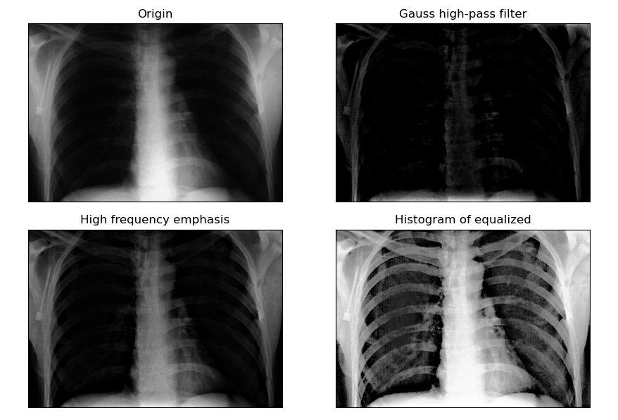
Routine 8.26: frequency domain passivation masking
    # 8.26: frequency domain passivation masking
    def gaussHighPassFilter(shape, radius=10):  # Gaussian Highpass Filter
        # Gaussian filter:# Gauss = 1/(2*pi*s2) * exp(-(x**2+y**2)/(2*s2))
        u, v = np.mgrid[-1:1:2.0/shape[0], -1:1:2.0/shape[1]]
        D = np.sqrt(u**2 + v**2)
        D0 = radius / shape[0]
        kernel = 1 - np.exp(- (D ** 2) / (2 *D0**2))
        return kernel

    def dft2Image(image):  #Optimal extended fast Fourier transform
        # Centralized 2D array f (x, y) * - 1 ^ (x + y)
        mask = np.ones(image.shape)
        mask[1::2, ::2] = -1
        mask[::2, 1::2] = -1
        fImage = image * mask  # f(x,y) * (-1)^(x+y)

        # Optimal DFT expansion size
        rows, cols = image.shape[:2]  # The height and width of the original picture
        rPadded = cv2.getOptimalDFTSize(rows)  # Optimal DFT expansion size
        cPadded = cv2.getOptimalDFTSize(cols)  # For fast Fourier transform

        # Edge extension (complement 0), fast Fourier transform
        dftImage = np.zeros((rPadded, cPadded, 2), np.float32)  # Edge expansion of the original image
        dftImage[:rows, :cols, 0] = fImage  # Edge expansion, 0 on the lower and right sides
        cv2.dft(dftImage, dftImage, cv2.DFT_COMPLEX_OUTPUT)  # fast Fourier transform
        return dftImage


    # High frequency filtering + histogram equalization
    image = cv2.imread("../images/Fig0459a.tif", flags=0)  # flags=0 read as grayscale image
    rows, cols = image.shape[:2]  # The height and width of the picture
    print(rows, cols)

    # fast Fourier transform
    dftImage = dft2Image(image)  # Fast Fourier transform (rPad, cPad, 2)
    rPadded, cPadded = dftImage.shape[:2]  # Fast Fourier transform size, original image size optimization
    # Construct Gaussian low pass filter
    hpFilter = gaussHighPassFilter((rPadded, cPadded), radius=10)  # Gaussian Highpass Filter
    # Modify Fourier transform in frequency domain: Fourier transform point multiplication low-pass filter
    dftHPfilter = np.zeros(dftImage.shape, dftImage.dtype)  # Size of fast Fourier transform (optimized size)
    for j in range(2):
        dftHPfilter[:rPadded, :cPadded, j] = dftImage[:rPadded, :cPadded, j] * hpFilter
    # The inverse Fourier transform is performed on the high pass Fourier transform and only the real part is taken
    idft = np.zeros(dftImage.shape[:2], np.float32)  # Size of fast Fourier transform (optimized size)
    cv2.dft(dftHPfilter, idft, cv2.DFT_REAL_OUTPUT + cv2.DFT_INVERSE + cv2.DFT_SCALE)
    # Centralized 2D array g (x, y) * - 1 ^ (x + y)
    mask2 = np.ones(dftImage.shape[:2])
    mask2[1::2, ::2] = -1
    mask2[::2, 1::2] = -1
    idftCen = idft * mask2  # g(x,y) * (-1)^(x+y)
    # Intercept the upper left corner, the size is equal to the input image
    result = np.clip(idftCen, 0, 255)  # Truncation function, limiting the value to [0255]
    imgHPF = result.astype(np.uint8)
    imgHPF = imgHPF[:rows, :cols]

    # # =======High frequency enhanced filtering===================
    k1 = 0.5
    k2 = 0.75
    # Modify Fourier transform in frequency domain: Fourier transform point multiplication low-pass filter
    hpEnhance = np.zeros(dftImage.shape, dftImage.dtype)  # Size of fast Fourier transform (optimized size)
    for j in range(2):
        hpEnhance[:rPadded, :cPadded, j] = dftImage[:rPadded, :cPadded, j] * (k1 + k2*hpFilter)
    # The inverse Fourier transform is performed on the high pass Fourier transform and only the real part is taken
    idft = np.zeros(dftImage.shape[:2], np.float32)  # Size of fast Fourier transform (optimized size)
    cv2.dft(hpEnhance, idft, cv2.DFT_REAL_OUTPUT + cv2.DFT_INVERSE + cv2.DFT_SCALE)
    # Centralized 2D array g (x, y) * - 1 ^ (x + y)
    mask2 = np.ones(dftImage.shape[:2])
    mask2[1::2, ::2] = -1
    mask2[::2, 1::2] = -1
    idftCen = idft * mask2  # g(x,y) * (-1)^(x+y)
    # Intercept the upper left corner, the size is equal to the input image
    result = np.clip(idftCen, 0, 255)  # Truncation function, limiting the value to [0255]
    imgHPE= result.astype(np.uint8)
    imgHPE = imgHPE[:rows, :cols]

    # =======Histogram equalization===================
    imgEqu = cv2.equalizeHist(imgHPE)  # Use CV2 Equalizehist completes histogram equalization transformation

    plt.figure(figsize=(9, 6))
    plt.subplot(221), plt.imshow(image, 'gray'), plt.title("Origin"), plt.xticks([]), plt.yticks([])
    plt.subplot(222), plt.imshow(imgHPF, 'gray'), plt.title("Gauss high-pass filter"), plt.xticks([]), plt.yticks([])
    plt.subplot(223), plt.imshow(imgHPE, 'gray'), plt.title("High frequency emphasis"), plt.xticks([]), plt.yticks([])
    plt.subplot(224), plt.imshow(imgEqu, 'gray'), plt.title("Histogram of equalized"), plt.xticks([]), plt.yticks([])
    plt.tight_layout()
    plt.show()
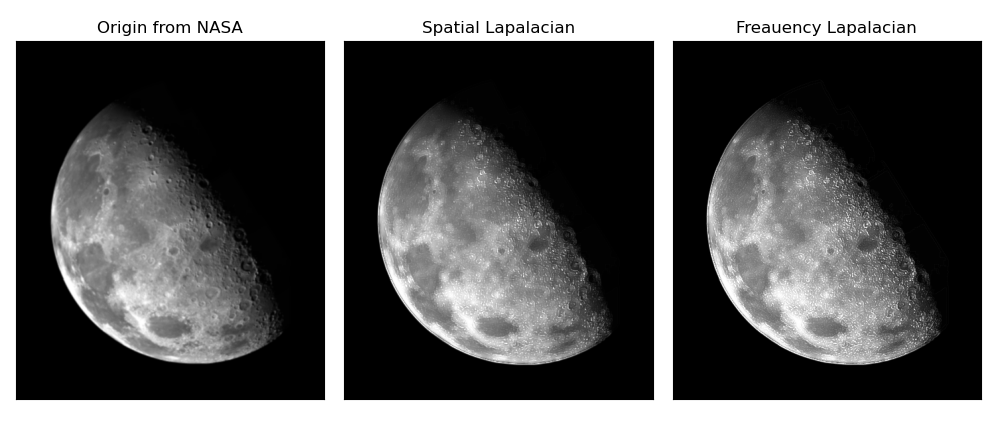
4.3 Laplace high pass filtering in frequency domain
Laplace operator is a derivative operator, which will highlight the sharp gray change in the image and suppress the slow gray change area. It often produces gray edges and discontinuous images under dark background. By superimposing the Laplacian image with the original image, the image with the sharpening effect can be obtained.
Laplace operator is the simplest isotropic derivative operator (convolution kernel):
∇
2
f
=
∂
2
f
∂
x
2
+
∂
2
f
∂
y
2
∂
2
f
∂
x
2
=
f
(
x
+
1
,
y
)
−
2
f
(
x
,
y
)
+
f
(
x
−
1
,
y
)
∂
2
f
∂
y
2
=
f
(
x
,
y
+
1
)
−
2
f
(
x
,
y
)
+
f
(
x
,
y
−
1
)
∇
2
f
(
x
,
y
)
=
f
(
x
+
1
,
y
)
+
f
(
x
−
1
,
y
)
+
f
(
x
,
y
+
1
)
+
f
(
x
,
y
−
1
)
−
4
f
(
x
,
y
)
\begin{aligned} \nabla ^2 f &= \dfrac{\partial ^2 f}{\partial x ^2} + \dfrac{\partial ^2 f}{\partial y ^2} \\ \dfrac{\partial ^2 f}{\partial x ^2} &= f(x+1,y) - 2f(x,y) + f(x-1,y) \\ \dfrac{\partial ^2 f}{\partial y ^2} &= f(x,y+1) - 2f(x,y) + f(x,y-1) \\ \nabla ^2 f(x,y) &= f(x+1,y) + f(x-1,y) + f(x,y+1) + f(x,y-1) - 4f(x,y) \end{aligned}
∇2f∂x2∂2f∂y2∂2f∇2f(x,y)=∂x2∂2f+∂y2∂2f=f(x+1,y)−2f(x,y)+f(x−1,y)=f(x,y+1)−2f(x,y)+f(x,y−1)=f(x+1,y)+f(x−1,y)+f(x,y+1)+f(x,y−1)−4f(x,y)
Therefore, the Laplace kernel K1 in the spatial domain can be obtained, and the Laplace kernel K2 can be obtained after considering the diagonal term.
K 1 = [ 0 1 0 1 − 4 1 0 1 0 ] , K 2 = [ 1 1 1 1 − 8 1 1 1 1 ] , K 3 = [ 0 − 1 0 − 1 4 − 1 0 − 1 0 ] , K 4 = [ − 1 − 1 − 1 − 1 8 − 1 − 1 − 1 − 1 ] K1= \begin{bmatrix} 0 & 1 &0\\ 1 & -4 &1\\ 0 & 1 &0\\ \end{bmatrix}, \ K2= \begin{bmatrix} 1 & 1 &1\\ 1 & -8 &1\\ 1 & 1 &1\\ \end{bmatrix}, \ K3= \begin{bmatrix} 0 & -1 &0\\ -1 & 4 &-1\\ 0 & -1 &0\\ \end{bmatrix}, \ K4= \begin{bmatrix} -1 & -1 &-1\\ -1 & 8 &-1\\ -1 & -1 &-1\\ \end{bmatrix} K1=⎣⎡0101−41010⎦⎤, K2=⎣⎡1111−81111⎦⎤, K3=⎣⎡0−10−14−10−10⎦⎤, K4=⎣⎡−1−1−1−18−1−1−1−1⎦⎤
In the frequency domain, Laplacian can be described by transfer function:
H
(
u
,
v
)
=
−
4
π
2
(
u
2
+
v
2
)
H(u,v) = - 4 \pi ^2 (u^2 + v^2)
H(u,v)=−4π2(u2+v2)
D(u,v) is used to represent the distance function from the frequency center, which can be further expressed as:
H
(
u
,
v
)
=
−
4
π
2
[
(
u
−
P
/
2
)
2
+
(
v
−
Q
/
2
)
2
]
=
−
4
π
2
D
2
(
u
,
v
)
H(u,v) = - 4 \pi ^2 [(u-P/2)^2 + (v-Q/2)^2] = - 4 \pi ^2 D^2(u,v)
H(u,v)=−4π2[(u−P/2)2+(v−Q/2)2]=−4π2D2(u,v)
therefore,
KaTeX parse error: No such environment: align at position 8: \begin{̲a̲l̲i̲g̲n̲}̲ \nabla ^2 f(x,...
Routine 8.27: frequency domain image sharpening (Laplace operator)
    # 8.27: image sharpening in frequency domain (Laplace operator)
    def LaplacianFilter(shape):  # Frequency domain Laplacian filter
        u, v = np.mgrid[-1:1:2.0/shape[0], -1:1:2.0/shape[1]]
        D = np.sqrt(u**2 + v**2)
        kernel = -4 * np.pi**2 * D**2
        return kernel

    def imgHPfilter(image, lpTyper="Laplacian"):  #Frequency domain high pass filtering
        # (1) Centralized 2D array f (x, y) * - 1 ^ (x + y)
        mask = np.ones(image.shape)
        mask[1::2, ::2] = -1
        mask[::2, 1::2] = -1
        fImage = image * mask  # f(x,y) * (-1)^(x+y)

        # (2) Optimal DFT expansion size, size expansion of fast Fourier transform
        rows, cols = image.shape[:2]  # The height and width of the original picture
        rPadded = cv2.getOptimalDFTSize(rows)  # Optimal DFT expansion size
        cPadded = cv2.getOptimalDFTSize(cols)  # For fast Fourier transform

        # (3) Edge extension (complement 0), fast Fourier transform
        dftImage = np.zeros((rPadded, cPadded, 2), np.float32)  # Edge expansion of the original image
        dftImage[:rows, :cols, 0] = fImage  # Edge expansion, 0 on the lower and right sides
        cv2.dft(dftImage, dftImage, cv2.DFT_COMPLEX_OUTPUT)  # Fast Fourier transform (rPad, cPad, 2)

        # (4) Constructing frequency domain filter transfer function: Taking Laplacian as an example
        LapFilter = LaplacianFilter((rPadded, cPadded))  # Laplacian filter

        # (5) Modify Fourier transform in frequency domain: Fourier transform point multiplication filter transfer function
        dftFilter = np.zeros(dftImage.shape, dftImage.dtype)  # Size of fast Fourier transform (optimized size)
        for j in range(2):
            dftFilter[:rPadded, :cPadded, j] = dftImage[:rPadded, :cPadded, j] * LapFilter

        # (6) The high pass Fourier transform is performed only on the inverse part
        idft = np.zeros(dftImage.shape[:2], np.float32)  # Size of fast Fourier transform (optimized size)
        cv2.dft(dftFilter, idft, cv2.DFT_REAL_OUTPUT + cv2.DFT_INVERSE + cv2.DFT_SCALE)

        # (7) Centralized 2D array g (x, y) * - 1 ^ (x + y)
        mask2 = np.ones(dftImage.shape[:2])
        mask2[1::2, ::2] = -1
        mask2[::2, 1::2] = -1
        idftCen = idft * mask2  # g(x,y) * (-1)^(x+y)

        # (8) Intercept the upper left corner, the size is equal to the input image
        result = np.clip(idftCen, 0, 255)  # Truncation function, limiting the value to [0255]
        imgFilter = result.astype(np.uint8)
        imgFilter = imgFilter[:rows, :cols]
        return imgFilter


    # (1) Read original image
    img = cv2.imread("../images/Fig0338a.tif", flags=0)  # NASA lunar image
    rows, cols = img.shape[:2]  # The height and width of the picture
    print(rows, cols)

    # (2) Laplacian in space domain
    # Implementation of Laplace convolution operator using function filter2D
    kernLaplace = np.array([[0, 1, 0], [1, -4, 1], [0, 1, 0]])  # Laplacian kernel
    imgLaplace1 = cv2.filter2D(img, -1, kernLaplace, borderType=cv2.BORDER_REFLECT)
    # Use CV2 Laplacian implementation of Laplace convolution operator
    imgLaplace2 = cv2.Laplacian(img, -1, ksize=3)
    imgLapReSpace = cv2.add(img, imgLaplace2)  # Restore original image

    # (3) Laplacian in frequency domain
    imgLaplace = imgHPfilter(img, "Laplacian")  # Call the custom function imgHPfilter()
    imgLapRe = cv2.add(img, imgLaplace)  # Restore original image

    plt.figure(figsize=(10, 6))
    plt.subplot(131), plt.imshow(img, 'gray'), plt.title("Origin from NASA"), plt.xticks([]), plt.yticks([])
    plt.subplot(132), plt.imshow(imgLapReSpace, 'gray'), plt.title("Spatial Lapalacian"), plt.xticks([]), plt.yticks([])
    plt.subplot(133), plt.imshow(imgLapRe, 'gray'), plt.title("Freauency Lapalacian"), plt.xticks([]), plt.yticks([])
    plt.tight_layout()
    plt.show()
5. Selective filtering
5.1 band stop and band pass
Linear filters in space domain and frequency domain can be divided into four categories: low-pass filter, high pass filter, band-pass filter and band stop filter. Both high pass filtering and low-pass filtering operate on the whole frequency rectangle, while band-pass filtering and band stop filtering process specific frequency bands and belong to selective filtering.
The high pass filter in the frequency domain can be derived from the low-pass filter. Similarly, the transfer functions of band-pass and band stop filters in the frequency domain can be constructed by a combination of low-pass filters and high pass filters.
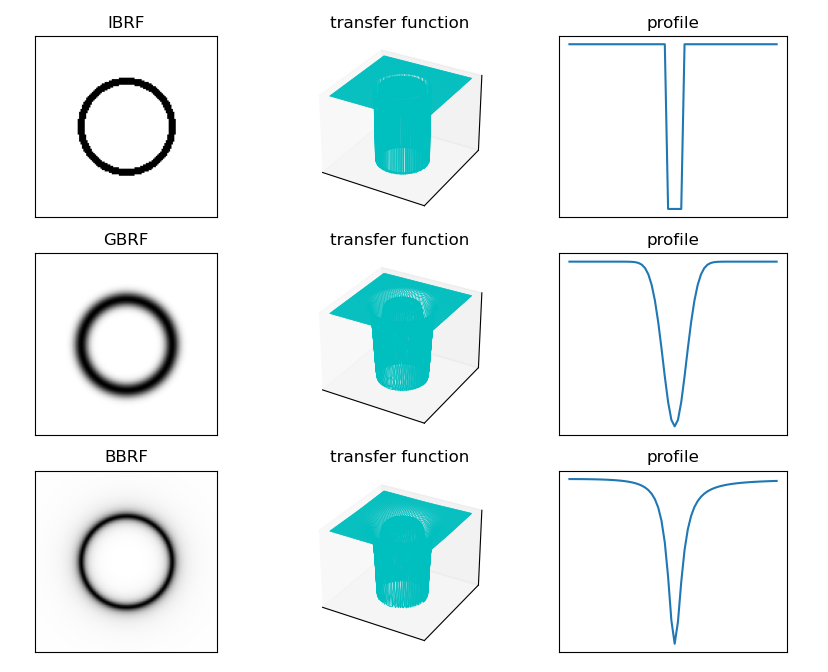
The transfer function of ideal band stop filter (IBRF) is:
H
(
u
,
v
)
=
{
0
,
(
C
0
−
W
/
2
)
≤
D
(
u
,
v
)
≤
(
C
0
+
W
/
2
)
1
,
e
l
s
e
H(u,v)=\begin{cases} 0,\ (C_0-W/2) \leq D(u,v) \leq (C_0+W/2)\\ 1,\ else \end{cases}
H(u,v)={0, (C0−W/2)≤D(u,v)≤(C0+W/2)1, else
The transfer function of Gaussian band stop filter (GBRF) is:
H
(
u
,
v
)
=
1
−
e
−
[
D
2
(
u
,
v
)
−
C
0
2
D
(
u
,
v
)
W
]
2
H(u,v)=1-e^{-[ \frac {D^2(u,v) - C_0^2} {D(u,v)W}]^2}
H(u,v)=1−e−[D(u,v)WD2(u,v)−C02]2
**The transfer function of Butterworth band stop filter (BBRF) is:**
H
(
u
,
v
)
=
1
1
+
[
D
(
u
,
v
)
W
D
2
(
u
,
v
)
−
C
0
2
]
2
n
H(u,v)= \frac {1} {1 +[ \frac {D(u,v)W} {D^2(u,v) - C_0^2}]^{2n}}
H(u,v)=1+[D2(u,v)−C02D(u,v)W]2n1
Routine 8.28 transfer function of band stop filter
    # Routine 8.28 transfer function of band stop filter
    def ideaBondResistFilter(shape, radius=10, w=5):  # Ideal band stop filter
        u, v = np.meshgrid(np.arange(shape[1]), np.arange(shape[0]))
        D = np.sqrt((u - shape[1]//2)**2 + (v - shape[0]//2)**2)
        D0 = radius
        halfW = w/2
        kernel = np.piecewise(D, [D<=D0+halfW, D<=D0-halfW], [1, 0])
        kernel = 1 - kernel  # Band stop
        return kernel

    def gaussBondResistFilter(shape, radius=10, w=5):  # Gaussian band stop filter
        # Gaussian filter:# Gauss = 1/(2*pi*s2) * exp(-(x**2+y**2)/(2*s2))
        u, v = np.meshgrid(np.arange(shape[1]), np.arange(shape[0]))
        D = np.sqrt((u - shape[1]//2)**2 + (v - shape[0]//2)**2)
        C0 = radius
        kernel = 1 - np.exp(-(D-C0)**2 / (w**2))
        return kernel

    def butterworthBondResistFilter(shape, radius=10, w=5, n=1):  # Butterworth band stop filter
        u, v = np.meshgrid(np.arange(shape[1]), np.arange(shape[0]))
        D = np.sqrt((u - shape[1]//2)**2 + (v - shape[0]//2)**2)
        C0 = radius
        epsilon = 1e-8  # Prevent division by 0
        kernel = 1.0 / (1.0 + np.power(D*w/(D**2-C0**2+epsilon), 2*n))
        return kernel

    # Ideal, Gaussian, Butterworth band stop filter transfer function
    shape = [128, 128]
    radius = 32
    IBRF = ideaBondResistFilter(shape, radius=radius)
    GBRF = gaussBondResistFilter(shape, radius=radius)
    BBRF = butterworthBondResistFilter(shape, radius=radius)

    filters = ["IBRF", "GBRF", "BBRF"]
    u, v = np.mgrid[-1:1:2.0/shape[0], -1:1:2.0/shape[1]]
    fig = plt.figure(figsize=(10, 8))
    for i in range(3):
        hpFilter = eval(filters[i]).copy()

        ax1 = fig.add_subplot(3, 3, 3*i+1)
        ax1.imshow(hpFilter, 'gray')
        ax1.set_title(filters[i]), ax1.set_xticks([]), ax1.set_yticks([])

        ax2 = plt.subplot(3,3,3*i+2, projection='3d')
        ax2.set_title("transfer function")
        ax2.plot_wireframe(u, v, hpFilter, rstride=2, linewidth=0.5, color='c')
        ax2.set_xticks([]), ax2.set_yticks([]), ax2.set_zticks([])

        ax3 = plt.subplot(3,3,3*i+3)
        profile = hpFilter[shape[0]//2:, shape[1]//2]
        ax3.plot(profile), ax3.set_title("profile"), ax3.set_xticks([]), ax3.set_yticks([])

    plt.show()
5.2 Notch Filter
Notch filter blocks or passes through the frequency in the rectangular neighborhood of the predetermined frequency, which is an important selective filter.
Notch filter is a filter that can rapidly attenuate the input signal at a certain frequency point to achieve the filtering effect of hindering the passage of this frequency signal. Notch filter is a kind of band stop filter. Its stop band is very narrow, and the starting order must be more than second order (including second order).
The zero phase shift filter must give symmetry to the origin (the center of the frequency rectangle), so the center is ( u 0 , v 0 ) (u_0,v_0) The notch filter transfer function of (u0, v0) is ( − u 0 , − v 0 ) (-u_0, -v_0) (− u0, − v0) position must have a corresponding notch.
The transfer function of the notch band stop filter can be constructed by the product of the high pass filter whose center has been shifted to the center of the notch filter:
H
N
R
(
u
,
v
)
=
∏
k
=
1
Q
H
k
(
u
,
v
)
H
−
k
(
u
,
v
)
H_{NR}(u,v) = \prod_{k=1}^Q H_k(u,v) H_{-k}(u,v)
HNR(u,v)=k=1∏QHk(u,v)H−k(u,v)
The distance calculation formula of the filter is:
D
k
(
u
,
v
)
=
(
u
−
M
/
2
−
u
k
)
2
+
(
v
−
N
/
2
−
v
k
)
2
D
−
k
(
u
,
v
)
=
(
u
−
M
/
2
+
u
k
)
2
+
(
v
−
N
/
2
+
v
k
)
2
D_k(u,v) = \sqrt{(u-M/2-u_k)^2 + (v-N/2-v_k)^2} \\ D_{-k}(u,v) = \sqrt{(u-M/2+u_k)^2 + (v-N/2+v_k)^2}
Dk(u,v)=(u−M/2−uk)2+(v−N/2−vk)2
D−k(u,v)=(u−M/2+uk)2+(v−N/2+vk)2
For example, the n-order Butterworth notch band stop filter with 3 notch pairs is:
H
N
R
(
u
,
v
)
=
∏
k
=
1
3
[
1
1
+
[
D
0
k
/
D
k
(
u
,
v
)
]
n
]
[
1
1
+
[
D
−
k
/
D
k
(
u
,
v
)
]
n
]
H_{NR}(u,v) = \prod_{k=1}^3 [\frac{1}{1+[D_{0k}/D_k(u,v)]^n}] [\frac{1}{1+[D_{-k}/D_k(u,v)]^n}]
HNR(u,v)=k=1∏3[1+[D0k/Dk(u,v)]n1][1+[D−k/Dk(u,v)]n1]
The notch transfer function of the passband filter can be obtained:
H
N
P
(
u
,
v
)
=
1
−
H
N
R
(
u
,
v
)
H_{NP}(u,v) = 1 - H_{NR}(u,v)
HNP(u,v)=1−HNR(u,v)
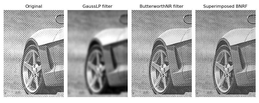
Routine 8.29 uses notch filtering to delete moire patterns in digital printed images
This example uses notch filtering to reduce the moire ripple in the digital printed image.
Moire pattern is the expression of beat difference principle. After the superposition of two equal amplitude sine waves with similar frequencies, the signal amplitude will change according to the difference between the two frequencies. If the spatial frequency of the pixel of the photosensitive element is close to the spatial frequency of the stripe in the image, the moire will be generated.
Notch filtering is to selectively modify the local region of DFT. The typical processing method is interactive operation. Directly use the mouse to select the rectangular region in the Fourier spectrum and find the maximum point as (uk,vk). In order to simplify the program, this routine deletes the mouse interaction part and only retains the filtering process after (uk,vk).
    # Routine 8.29 uses notch filtering to delete moire patterns in digital printed images

    def gaussLowPassFilter(shape, radius=10):  # Gaussian low pass filter
        u, v = np.mgrid[-1:1:2.0 / shape[0], -1:1:2.0 / shape[1]]
        D = np.sqrt(u ** 2 + v ** 2)
        D0 = radius / shape[0]
        kernel = np.exp(- (D ** 2) / (2 * D0 ** 2))
        return kernel

    def butterworthNRFilter(shape, radius=9, uk=60, vk=80, n=2):  # Butterworth notch band stop filter
        M, N = shape[1], shape[0]
        u, v = np.meshgrid(np.arange(M), np.arange(N))
        Dm = np.sqrt((u - M // 2 - uk) ** 2 + (v - N // 2 - vk) ** 2)
        Dp = np.sqrt((u - M // 2 + uk) ** 2 + (v - N // 2 + vk) ** 2)
        D0 = radius
        n2 = n * 2
        kernel = (1 / (1 + (D0 / (Dm + 1e-6)) ** n2)) * (1 / (1 + (D0 / (Dp + 1e-6)) ** n2))
        return kernel

    def imgFrequencyFilter(img, lpTyper="GaussLP", radius=10):
        normalize = lambda x: (x - x.min()) / (x.max() - x.min() + 1e-8)

        # (1) Edge fill
        imgPad = np.pad(img, ((0, img.shape[0]), (0, img.shape[1])), mode="reflect")
        # (2) Centralization: F (x, y) * - 1 ^ (x + y)
        mask = np.ones(imgPad.shape)
        mask[1::2, ::2] = -1
        mask[::2, 1::2] = -1
        imgPadCen = imgPad * mask
        # (3) Fourier transform
        fft = np.fft.fft2(imgPadCen)

        # (4) Construct the frequency domain filter transfer function:
        if lpTyper == "GaussLP":
            print(lpTyper)
            freFilter = gaussLowPassFilter(imgPad.shape, radius=60)
        elif lpTyper == "GaussHP":
            freFilter = gaussLowPassFilter(imgPad.shape, radius=60)
        elif lpTyper == "ButterworthNR":
            print(lpTyper)
            freFilter = butterworthNRFilter(imgPad.shape, radius=9, uk=60, vk=80, n=2)  # Butterworth notch band stop filter
        elif lpTyper == "MButterworthNR":
            print(lpTyper)
            BNRF1 = butterworthNRFilter(imgPad.shape, radius=9, uk=60, vk=80, n=2)  # Butterworth notch band stop filter
            BNRF2 = butterworthNRFilter(imgPad.shape, radius=9, uk=-60, vk=80, n=2)
            BNRF3 = butterworthNRFilter(imgPad.shape, radius=9, uk=60, vk=160, n=2)
            BNRF4 = butterworthNRFilter(imgPad.shape, radius=9, uk=-60, vk=160, n=2)
            freFilter = BNRF1 * BNRF2 * BNRF3 * BNRF4
        else:
            print("Error of unknown filter")
            return -1

        # (5) Modify Fourier transform in frequency domain: Fourier transform point multiplication filter transfer function
        freTrans = fft * freFilter
        # (6) Inverse Fourier transform
        ifft = np.fft.ifft2(freTrans)
        # (7) Decentralized inverse transform image
        M, N = img.shape[:2]
        mask2 = np.ones(imgPad.shape)
        mask2[1::2, ::2] = -1
        mask2[::2, 1::2] = -1
        ifftCenPad = ifft.real * mask2
        # (8) Intercept the upper left corner, the size is equal to the input image
        imgFilter = ifftCenPad[:M, :N]
        imgFilter = np.clip(imgFilter, 0, imgFilter.max())
        imgFilter = np.uint8(normalize(imgFilter) * 255)
        return imgFilter


    # Using notch filtering to delete moire patterns in digital printed images
    # (1) Read original image
    img = cv2.imread("../images/Fig0464a.tif", flags=0)  # flags=0 read as grayscale image
    fig = plt.figure(figsize=(10, 5))
    plt.subplot(141), plt.title("Original"), plt.axis('off'), plt.imshow(img, cmap='gray')

    # (2) Image Gaussian low pass filtering
    imgGLPF = imgFrequencyFilter(img, lpTyper="GaussLP", radius=30)  # Image Gaussian low pass filtering
    plt.subplot(142), plt.title("GaussLP filter"), plt.axis('off'), plt.imshow(imgGLPF, cmap='gray')

    # (3) Image Butterworth notch band stop filtering
    imgBNRF = imgFrequencyFilter(img, lpTyper="ButterworthNR", radius=9)
    plt.subplot(143), plt.title("ButterworthNR filter"), plt.axis('off'), plt.imshow(imgBNRF, cmap='gray')

    # (4) Superimposed Butterworth notch band stop filtering
    imgSBNRF = imgFrequencyFilter(img, lpTyper="MButterworthNR", radius=9)
    plt.subplot(144), plt.title("Superimposed BNRF"), plt.axis('off'), plt.imshow(imgSBNRF, cmap='gray')

    plt.tight_layout()
    plt.show()
Copyright notice:
Note: some of the original pictures in this article are from Rafael C. Gonzalez "Digital Image Processing, 4th.Ed." thank you.
OpenCV learning course for youcans Original works
Reprint must be marked with the original link: https://blog.csdn.net/youcans/article/details/122991620
Copyright 2021 youcans, XUPT
Crated: 2022-02-18
Welcome to pay attention "OpenCV learning course of youcans" Series, continuously updated
OpenCV learning course of youcans - 1 Installation and environment configuration
OpenCV learning course of youcans - 2 Image reading and display
OpenCV learning course of youcans - 3 Image creation and modification
OpenCV learning course of youcans - 4 Image overlay and blending
OpenCV learning course of youcans - 5 Geometric transformation of image
OpenCV learning course of youcans - 6 Gray transformation and histogram processing
OpenCV learning course of youcans - 7 Spatial domain image filtering
youcans OpenCV learning course - 8 Frequency domain image filtering (I)
youcans OpenCV learning course - 9 Frequency domain image filtering (Part 2)